User:Tohline/SSC/Virial/PolytropesEmbedded/SecondEffortAgain
Virial Equilibrium of Adiabatic Spheres (Summary)
The summary presented here has been drawn from our accompanying detailed analysis of the structure of pressure-truncated polytropes.

|
|---|
| | Tiled Menu | Tables of Content | Banner Video | Tohline Home Page | |
Detailed Force-Balanced Solution
As has been discussed in detail in another chapter, Horedt (1970), Whitworth (1981) and Stahler (1983) have separately derived what the equilibrium radius, <math>~R_\mathrm{eq}</math>, is of a polytropic sphere that is embedded in an external medium of pressure, <math>~P_e</math>. Their solution of the detailed force-balanced equations provides a pair of analytic expressions for <math>~R_\mathrm{eq}</math> and <math>~P_e</math> that are parametrically related to one another through the Lane-Emden function, <math>~\theta</math>, and its radial derivative. For example — see our related discussion for more details — from Horedt's work we obtain the following pair of equations:
|
<math> ~\frac{R_\mathrm{eq}}{R_\mathrm{norm}} = r_a \cdot \biggl( \frac{R_\mathrm{Horedt}}{R_\mathrm{norm}} \biggr) </math> |
<math>~=~</math> |
<math> \tilde\xi ( -\tilde\xi^2 \tilde\theta' )^{(1-n)/(n-3)} \biggl[ \frac{4\pi}{(n+1)^n} \biggl( \frac{M_\mathrm{limit}}{M_\mathrm{tot}}\biggr)^{n-1} \biggr]^{1/(n-3)} \, , </math> |
|
<math> ~\frac{P_\mathrm{e}}{P_\mathrm{norm}} = p_a \cdot \biggl( \frac{P_\mathrm{Horedt}}{P_\mathrm{norm}} \biggr) </math> |
<math>~=~</math> |
<math> \tilde\theta^{n+1}( -\tilde\xi^2 \tilde\theta' )^{2(n+1)/(n-3)} \biggl[ \frac{(n+1)^3}{4\pi} \biggl( \frac{M_\mathrm{limit}}{M_\mathrm{tot}} \biggr)^{-2}\biggr]^{(n+1)/(n-3)} \, , </math> |
where we have introduced the normalizations,
|
<math>~R_\mathrm{norm}</math> |
<math>~\equiv</math> |
<math>~\biggl[ \biggl( \frac{G}{K} \biggr)^n M_\mathrm{tot}^{n-1} \biggr]^{1/(n-3)} \, ,</math> |
|
<math>~P_\mathrm{norm}</math> |
<math>~\equiv</math> |
<math>~\biggl[ \frac{K^{4n}}{G^{3(n+1)} M_\mathrm{tot}^{2(n+1)}} \biggr]^{1/(n-3)} \, .</math> |
In the expressions for <math>~r_a</math> and <math>~p_a</math>, the tilde indicates that the Lane-Emden function and its derivative are to be evaluated, not at the radial coordinate, <math>~\xi_1</math>, that is traditionally associated with the "first zero" of the Lane-Emden function and therefore with the surface of the isolated polytrope, but at the radial coordinate, <math>~\tilde\xi</math>, where the internal pressure of the isolated polytrope equals <math>~P_e</math> and at which the embedded polytrope is to be truncated. The coordinate, <math>~\tilde\xi</math>, therefore identifies the surface of the embedded — or, pressure-truncated — polytrope. We also have taken the liberty of attaching the subscript "limit" to <math>~M</math> in both defining relations because it is clear that Horedt intended for the normalization mass to be the mass of the pressure-truncated object, not the mass of the associated isolated (and untruncated) polytrope.
From these previously published works, it is not obvious how — or even whether — this pair of parametric equations can be combined to directly show how the equilibrium radius depends on the value of the external pressure. Our examination of the free-energy of these configurations and, especially, an application of the viral theorem shows this direct relationship. Foreshadowing these results, we note that,
|
<math>~\biggl[ \biggl(\frac{P_e}{P_\mathrm{norm}}\biggr) \biggl(\frac{R_\mathrm{eq}}{R_\mathrm{norm}} \biggr)^4\biggr]_\mathrm{Horedt} </math> |
<math>~=</math> |
<math> \biggl[ \frac{\tilde\theta^{n+1} }{(4\pi)(n+1)( -\tilde\theta' )^{2}} \biggr] \biggl( \frac{M_\mathrm{limit}}{M_\mathrm{tot}}\biggr)^{2} \, ; </math> |
or, given that <math>~P_\mathrm{norm}R_\mathrm{norm}^4 = GM_\mathrm{tot}^2</math>, this can be rewritten as,
|
<math>~\biggl[ \frac{P_e R_\mathrm{eq}^4}{G M_\mathrm{limit}^2} \biggr]_\mathrm{Horedt} </math> |
<math>~=</math> |
<math> \frac{\tilde\theta^{n+1} }{(4\pi)(n+1)( -\tilde\theta' )^{2}} \, . </math> |
Free Energy Function and Virial Theorem
The variation with size of the normalized free energy, <math>~\mathfrak{G}^*</math>, of pressure-truncated adiabatic spheres is described by the following,
Algebraic Free-Energy Function
<math> \mathfrak{G}^* = -3\mathcal{A} \chi^{-1} +~ \frac{1}{(\gamma - 1)} \mathcal{B} \chi^{3-3\gamma} +~ \mathcal{D}\chi^3 \, . </math>
In this expression, the size of the configuration is set by the value of the dimensionless radius, <math>~\chi \equiv R/R_\mathrm{norm}</math>; as is clarified, below, the values of the coefficients, <math>~\mathcal{A}</math> and <math>~\mathcal{B}</math>, characterize the relative importance, respectively, of the gravitational potential energy and the internal thermal energy of the configuration; <math>~\gamma</math> is the exponent (from the adopted equation of state) that identifies the adiabat along which the configuration heats or cools upon expansion or contraction; and the relative importance of the imposed external pressure is expressed through the free-energy expression's third constant coefficient, specifically,
<math>~\mathcal{D} \equiv \frac{4\pi}{3} \biggl( \frac{P_e}{P_\mathrm{norm}} \biggr) \, .</math>
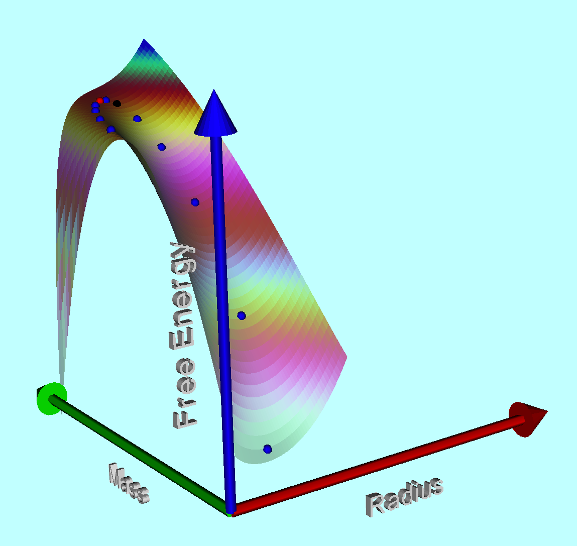
When examining a range of physically reasonable configuration sizes for a given choice of the constants <math>~(\gamma, \mathcal{A}, \mathcal{B}, \mathcal{D})</math>, a plot of <math>~\mathfrak{G}^*</math> versus <math>~\chi</math> will often reveal one or two extrema. Each extremum is associated with an equilibrium radius, <math>~\chi_\mathrm{eq} \equiv R_\mathrm{eq}/R_\mathrm{norm}</math>.
Equilibrium radii may also be identified through an algebraic relation that originates from the scalar virial theorem — a theorem that, itself, is derivable from the free-energy expression by setting <math>~\partial\mathfrak{G}^*/\partial\chi = 0</math>. In our accompanying detailed analysis of the structure of pressure-truncated polytropes, we use the virial theorem to show that the equilibrium radii that are identified by extrema in the free-energy function always satisfy the following,
Algebraic Expression of the Virial Theorem
<math> \Pi_\mathrm{ad} = \frac{(\Chi_\mathrm{ad}^{4-3\gamma} - 1)}{\Chi_\mathrm{ad}^4} \, , </math>
where, after setting <math>~\gamma = (n+1)/n</math>,
|
<math>~\Pi_\mathrm{ad}</math> |
<math>~=</math> |
<math> ~\mathcal{D} \biggl[ \frac{\mathcal{A}^{3(n+1)}}{\mathcal{B}^{4n}} \biggr]^{1/(n-3)} \, , </math> and, |
|
<math>~\Chi_\mathrm{ad}</math> |
<math>~=</math> |
<math> ~\chi_\mathrm{eq} \biggl[ \frac{\mathcal{B}}{\mathcal{A}} \biggr]^{n/(n-3)} \, . </math> |
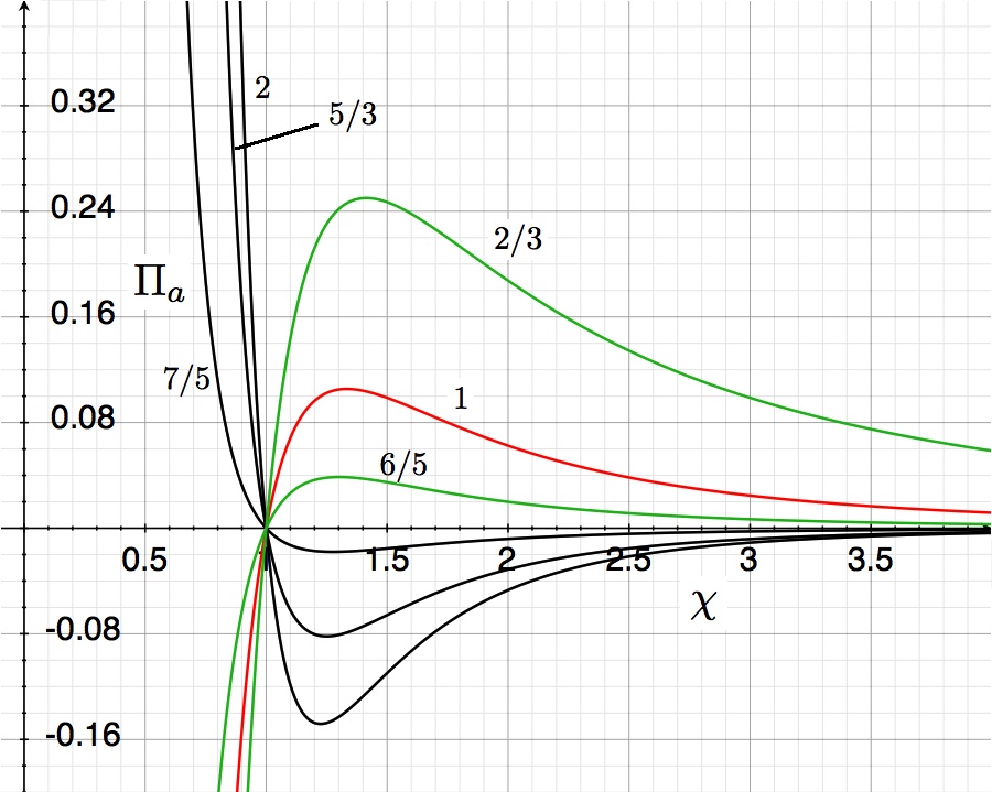
The curves shown in the accompanying "pressure-radius" diagram trace out this derived virial-theorem function for six different values of the adiabatic exponent, <math>~\gamma</math>, as labeled. They show the dimensionless external pressure, <math>~\Pi_\mathrm{ad}</math>, that is required to construct a nonrotating, self-gravitating, adiabatic sphere with a dimensionless equilibrium radius <math>~\Chi_\mathrm{ad}</math>. The mathematical solution becomes unphysical wherever the pressure becomes negative.
If we multiply the above free=energy function through by an appropriate combination of the coefficients, <math>~\mathcal{A}</math> and <math>~\mathcal{B}</math>, and make the substitution, <math>~\gamma \rightarrow (n+1)/n</math>, it also takes on a particularly simple form featuring the newly defined dimensionless external pressure, <math>~\Pi_\mathrm{ad}</math>, and the newly identified dimensionless radius, <math>~\Chi \equiv \chi(\mathcal{B}/\mathcal{A})^{n/(n-3)}</math>. Specifically, we obtain the,
Renormalized Free-Energy Function
<math> \mathfrak{G}^{**} \equiv \mathfrak{G}^* \biggl[ \frac{\mathcal{A}^3}{\mathcal{B}^n} \biggr]^{1/(n-3)} = -3 \Chi^{-1} +~ n\Chi^{-3/n} +~ \Pi_\mathrm{ad}\Chi^3 \, . </math>
Relationship to Detailed Force-Balanced Models
Structural Form Factors
In our accompanying detailed analysis, we demonstrate that the expressions given above for the free-energy function and the virial theorem are correct in sufficiently strict detail that they can be used to precisely match — and assist in understanding — the equilibrium of embedded polytropes whose structures have been determined from the set of detailed force-balance equations. In order to draw this association, it is only necessary to realize that, very broadly, the constant coefficients, <math>~\mathcal{A}</math> and <math>~\mathcal{B}</math>, in the above algebraic free-energy expression are expressible in terms of three structural form factors, <math>~\tilde\mathfrak{f}_M</math>, <math>~\tilde\mathfrak{f}_W</math>, and <math>~\tilde\mathfrak{f}_A</math>, as follows:
|
<math>~\mathcal{A}</math> |
<math>~\equiv</math> |
<math>\frac{1}{5} \cdot \biggl[ \biggl( \frac{M_\mathrm{limit}}{M_\mathrm{tot}} \biggr) \frac{1}{\tilde\mathfrak{f}_M} \biggr]^2 \cdot \tilde\mathfrak{f}_W \, ,</math> |
|
<math>~\mathcal{B}</math> |
<math>~\equiv</math> |
<math> \frac{4\pi}{3} \biggl[ \frac{3}{4\pi} \biggl( \frac{M_\mathrm{limit}}{M_\mathrm{tot}}\biggr) \frac{1}{\tilde\mathfrak{f}_M} \biggr]_\mathrm{eq}^{(n+1)/n} \cdot \tilde\mathfrak{f}_A = \frac{4\pi}{3} \biggl[ \biggl( \frac{P_c}{P_\mathrm{norm}} \biggr)\chi^{3(n+1)/n} \biggr]_\mathrm{eq} \cdot \tilde\mathfrak{f}_A \, ; </math> |
and that, specifically in the context of spherically symmetric, pressure-truncated polytropes, we can write …
|
Structural Form Factors for Pressure-Truncated Polytropes | ||||||
|---|---|---|---|---|---|---|
|
After plugging these nontrivial expressions for <math>~\mathcal{A}</math> and <math>~\mathcal{B}</math> into the righthand sides of the above equations for <math>~\Pi_\mathrm{ad}</math> and <math>~\Chi_\mathrm{ad}</math> and, simultaneously, using Horedt's detailed force-balanced expressions for <math>~r_a</math> and <math>~p_a</math> to specify, respectively, <math>~\chi_\mathrm{eq}</math> and <math>~P_e/P_\mathrm{norm}</math> in these same equations — see our accompanying discussion — we find that,
|
<math>~\Pi_\mathrm{ad}</math> |
<math>~=</math> |
<math>~\eta_\mathrm{ad} (1 + \eta_\mathrm{ad})^{-4n/(n-3)} \, ,</math> |
|
<math>~\Chi_\mathrm{ad}</math> |
<math>~=</math> |
<math>~(1 + \eta_\mathrm{ad})^{n/(n-3)} \, ,</math> |
where the newly identified, key physical parameter,
|
<math>~\eta_\mathrm{ad} \equiv \frac{b_\mathrm{ad}}{a_\mathrm{ad}}</math> |
<math>~=</math> |
<math>~\frac{3\cdot 5~ \tilde\theta^{n+1}}{(n+1) \tilde\xi^2 \mathfrak{f}_W} \, .</math> |
It is straightforward to show that this more compact pair of expressions for <math>~\Pi_\mathrm{ad}</math> and <math>~\Chi_\mathrm{ad}</math> satisfy the virial theorem presented above.
Physical Meaning of Parameter <math>~\eta_\mathrm{ad}</math>
In association with our accompanying derivation of a concise expression for the virial theorem, we see that the structural form factor associated with the thermal energy reservoir of our configuration is the sum of two terms, specifically,
<math>~\tilde\mathfrak{f}_A = a_\mathrm{ad} + b_\mathrm{ad} \, ,</math>
while, as defined in our above discussion, <math>~\eta_\mathrm{ad}</math> is the ratio of these same two terms, specifically,
<math>~\eta_\mathrm{ad} = \frac{b_\mathrm{ad}}{a_\mathrm{ad}} \, .</math>
It is worth pointing out what physical quantities are associated with these two terms.
At any radial location within a polytropic configuration, the Lane-Emden function, <math>~\theta</math>, is defined in terms of a ratio of the local density to the configuration's central density, specifically,
<math>\theta \equiv \biggl(\frac{\rho}{\rho_c} \biggr)^{1/n} \, .</math>
Remembering that, at any location within the configuration, the pressure is related to the density via the polytropic equation of state,
<math>P = K\rho^{(n+1)/n} \, ,</math>
we see that,
<math>\frac{P}{P_c} = \theta^{n+1} \, .</math>
Hence, the quantity, <math>~\tilde\theta^{n+1}</math>, which appears as the second term in our definition of <math>~\tilde\mathfrak{f}_A</math>, is the ratio, <math>~(P/P_c)_{\tilde\xi}</math>, evaluated at the surface of the truncated polytropic sphere. But, by construction, the pressure at this location equals the pressure of the external medium in which the polytrope is embedded, so we can write,
<math>b_\mathrm{ad} \equiv \tilde\theta^{n+1} = \frac{P_e}{P_c} \, .</math>
Also, directly from its integral definition, we have that <math>~\tilde\mathfrak{f}_A = \bar{P}/P_c</math>. So we can write,
|
<math>~a_\mathrm{ad}</math> |
<math>~=</math> |
<math>~\tilde\mathfrak{f}_A - b_\mathrm{ad } = \frac{\bar{P}}{P_c} - \frac{P_e}{P_c} = \frac{P_e}{P_c}\biggl( \frac{\bar{P}}{P_e} - 1 \biggr) \, .</math> |
We conclude, therefore, that,
<math>~\eta_\mathrm{ad} = \biggl( \frac{\bar{P}}{P_e} - 1 \biggr)^{-1} \, .</math>
Desired Pressure-Radius Relation
It is clear from the above discussion that the pair of parametric equations obtained via a solution of the detailed force-balanced equations satisfy our, slightly rearranged,
Algebraic Expression of the Virial Theorem
<math> \Pi_\mathrm{ad} \Chi_\mathrm{ad}^4 = \Chi_\mathrm{ad}^{(n-3)/n} - 1 \, . </math>
More to the point, it is now clear that this virial theorem expression provides the direct relationship between the configuration's dimensionless equilibrium radius as defined by Horedt, <math>~r_a</math>, and the dimensionless applied external pressure as defined by Horedt, <math>~p_a</math>, that was not apparent from the original pair of parametric relations. Horedt's parameters, <math>~r_a</math> and <math>~p_a</math>, can be directly associated to our parameters, <math>~\Chi_\mathrm{ad}</math> and <math>~\Pi_\mathrm{ad}</math>, via two new normalizations, <math>~r_n</math> and <math>~p_n</math>, defined through the relations,
|
<math>~\Chi_\mathrm{ad} = \frac{r_a}{r_n}</math> |
and |
<math>~\Pi_\mathrm{ad} = \frac{p_a}{p_n} \, .</math> |
Specifically in terms of the coefficients in the free-energy expression,
|
<math>~r_n^{n-3}</math> |
<math>~\equiv</math> |
<math>~ \frac{(n+1)^n}{4\pi} \biggl( \frac{M_\mathrm{limit}}{M_\mathrm{tot}} \biggr)^{1-n} \biggl( \frac{\mathcal{A}}{\mathcal{B}} \biggr)^n \, , </math> |
and,
|
<math>~p_n^{n-3}</math> |
<math>~\equiv</math> |
<math>~ \frac{3^{n-3}}{(4\pi)^4 (n+1)^{3(n+1)}} \biggl( \frac{M_\mathrm{limit}}{M_\mathrm{tot}} \biggr)^{2(n+1)} \biggl[ \frac{\mathcal{B}^{4n}}{\mathcal{A}^{3(n+1)}} \biggr] \, ; </math> |
while, in terms of the structural form factors,
|
<math>~r_n^{n-3}</math> |
<math>~\equiv</math> |
<math>~ \frac{1}{3} \biggl[ \frac{(n+1)}{5} \cdot \frac{\mathfrak{f}_W}{\mathfrak{f}_A} \biggr]^n \mathfrak{f}_M^{1-n} \, , </math> |
and,
|
<math>~p_n^{n-3}</math> |
<math>~\equiv</math> |
<math>~ \frac{1}{(4\pi)^8} \biggl[ \frac{3\cdot 5^3}{(n+1)^3} \cdot \frac{\mathfrak{f}_M^2}{\mathfrak{f}_W^3} \biggr]^{n+1} \mathfrak{f}_A^{4n} \, . </math> |
Implications Regarding Stability
Model Sequences
After choosing a value for the system's adiabatic index (or, equivalently, its polytropic index), <math>~\gamma = (n+1)/n</math>, the functional form of the virial theorem expression, <math>~\Pi_\mathrm{ad}(\chi_\mathrm{ad})</math>, is known and, hence, the equilibrium model sequence can be plotted. Half-a-dozen such model sequences are shown in the figure near the beginning of this discussion. Each curve can be viewed as mapping out a single-parameter sequence of equilibrium models; "evolution" along the curve can be accomplished by varying the key parameter, <math>~\eta_\mathrm{ad}</math>, over the physically relevant range, <math>0 \le \eta_\mathrm{ad} < \infty</math>.
|
ASIDE [18 March 2015]: Many months after I penned the above description of "evolution" along an equilibrium model sequence, I started analyzing in detail the paper by Kimura (1981b). The following excerpt from §3 of his paper shows that Kimura presented essentially the same description of "evolution along a sequence" several decades ago: Kimura uses the subscript "1" to denote the equilibrium value of any physical quantity "Q"; in the figure shown here, on the right, we are holding the equilibrium mass fixed while allowing the external pressure and the configuration volume to vary, so Kimura would say that the figure displays various "M_1 sequences." And, as is explained more fully in an accompanying discussion, his "truncation parameter" is essentially the same as our truncation radius — specifically, <math>~\zeta_1 = (n+1)^{1/2}\tilde\xi</math>. When projected onto our discussion, the physically relevant range of truncation parameter values is, <math>~0 \le \tilde\xi \le \xi_1</math>, where <math>~\xi_1</math> is the Lane-Emden radius of an isolated (unbounded) polytropic sphere. |
To simplify our discussion, here, we redisplay the above figure and repeat a few key algebraic relations.
|
<math>~\eta_\mathrm{ad} </math> |
<math>~\equiv</math> |
<math>~\frac{3\cdot 5 ~\tilde\theta^{n+1}}{(n+1) \tilde\xi^2 \tilde\mathfrak{f}_W} = \frac{\tilde\theta^{n+1}}{\tilde\theta^{n+1} + 3(\tilde\theta^')^2 - \tilde\mathfrak{f}_M \tilde\theta}\, ,</math> |
|
<math>~\Pi_\mathrm{ad}</math> |
<math>~=</math> |
<math>~\eta_\mathrm{ad} (1 + \eta_\mathrm{ad})^{-4n/(n-3)} \, ,</math> |
|
<math>~\Chi_\mathrm{ad}</math> |
<math>~=</math> |
<math>~(1 + \eta_\mathrm{ad})^{n/(n-3)} \, .</math> |
Note that the last expression for <math>~\eta_\mathrm{ad}</math> has been obtained after inserting the analytic expression for the structural form-factor, <math>~\tilde\mathfrak{f}_W</math> that — as has been explained in an accompanying discussion — we derived with the help of Viala & Horedt (1974).
Stability
Analysis of the free-energy function allows us to not only ascertain the equilibrium radius of isolated polytropes and pressure-truncated polytropic configurations, but also the relative stability of these configurations. We begin by repeating the,
Renormalized Free-Energy Function
<math> \mathfrak{G}^{**} = -3 \Chi^{-1} +~ n\Chi^{-3/n} +~ \Pi_\mathrm{ad}\Chi^3 \, . </math>
The first and second derivatives of <math>~\mathfrak{G}^{**}</math>, with respect to the dimensionless radius, <math>~\Chi</math>, are, respectively,
|
<math>~\frac{\partial\mathfrak{G}^{**}}{\partial\Chi}</math> |
<math>~=</math> |
<math>~3 \Chi^{-2} -3\Chi^{-(n+3)/n} + 3\Pi_\mathrm{ad} \Chi^2 \, ,</math> |
|
<math>~\frac{\partial^2\mathfrak{G}^{**}}{\partial\Chi^2}</math> |
<math>~=</math> |
<math>~-6 \Chi^{-3} + \frac{3(n+3)}{n} \Chi^{-(2n+3)/n} + 6\Pi_\mathrm{ad} \Chi \, .</math> |
As alluded to, above, equilibrium radii are identified by values of <math>~\Chi</math> that satisfy the equation, <math>\partial\mathfrak{G}^{**}/\partial\Chi = 0</math>. Specifically, marking equilibrium radii with the subscript "ad", they will satisfy the
Algebraic Expression of the Virial Theorem
<math> \Pi_\mathrm{ad} = \frac{\Chi_\mathrm{ad}^{(n-3)/n} - 1}{\Chi_\mathrm{ad}^4} \, . </math>
Dynamical stability then depends on the sign of the second derivative of <math>~\mathfrak{G}^{**}</math>, evaluated at the equilibrium radius; specifically, configurations will be stable if,
|
<math>~\frac{\partial^2\mathfrak{G}^{**}}{\partial\Chi^2}\biggr|_{\Chi_\mathrm{ad}}</math> |
<math>~></math> |
<math>~0 \, ,</math> (stable) |
and they will be unstable if, upon evaluation at the equilibrium radius, the sign of the second derivative is less than zero. Hence, isolated polytropes as well as pressure-truncated polytropic configurations will be stable if,
|
<math>~0</math> |
<math>~< </math> |
<math>~3 \Chi_\mathrm{ad}^{-3} \biggl[ - 2 + \frac{(n+3)}{n} \Chi_\mathrm{ad}^{(n-3)/n} + 2\Pi_\mathrm{ad} \Chi_\mathrm{ad}^4 \biggr]</math> |
|
|
<math>~< </math> |
<math>~3 \Chi_\mathrm{ad}^{-3} \biggl\{ \frac{(n+3)}{n} \Chi_\mathrm{ad}^{(n-3)/n} + 2[\Chi_\mathrm{ad}^{(n-3)/n} -1] - 2\biggr\}</math> |
|
|
<math>~< </math> |
<math>~3 \Chi_\mathrm{ad}^{-3} \biggl[ \frac{3(n+1)}{n} \Chi_\mathrm{ad}^{(n-3)/n} - 4\biggr]</math> |
|
<math>\Rightarrow~~~~\Chi_\mathrm{ad}</math> |
<math>~> </math> |
<math>~\biggl[ \frac{4n}{3(n+1)} \biggr]^{n/(n-3)} \, .</math> (stable) |
Reference to this stability condition proves to be simpler if we define the limiting configuration size as,
<math>~\Chi_\mathrm{min} \equiv \biggl[ \frac{4n}{3(n+1)} \biggr]^{n/(n-3)} \, ,</math>
and write the stability condition as,
<math>~\Chi_\mathrm{ad} > \Chi_\mathrm{min} \, .</math> (stable)
When examining the equilibrium sequences found in the upper-righthand quadrant of the figure at the top of this page — each corresponding to a different value of the polytropic index, <math>~n > 3</math> or <math>~n < 0</math> — we find that <math>~\Chi_\mathrm{min}</math> corresponds to the location along each sequence where the dimensionless external pressure, <math>~\Pi_\mathrm{ad}</math>, reaches a maximum. (Keeping in mind that the virial theorem defines each of these sequences, this statement of fact can be checked by identifying where the condition, <math>~\partial\Pi_\mathrm{ad}/\partial\Chi_\mathrm{ad} = 0</math>, occurs according to the algebraic expression of the virial theorem.) Hence, we conclude that, along each sequence, no equilibrium configurations exist for values of the dimensionless external pressure that are greater than,
|
<math>~\Pi_\mathrm{max}</math> |
<math>~\equiv</math> |
<math>~\Chi_\mathrm{min}^{-4} \biggl[ \Chi_\mathrm{min}^{(n-3)/n} - 1 \biggr] </math> |
|
|
<math>~=</math> |
<math>~\biggl[ \frac{3(n+1)}{4n} \biggr]^{4n/(n-3)} \biggl[\frac{4n}{3(n+1)} - 1 \biggr]</math> |
|
|
<math>~=</math> |
<math>~\biggl\{ \biggl[ \frac{3(n+1)}{4n} \biggr]^{4n} \biggl[\frac{n-3}{3(n+1)} \biggr]^{n-3} \biggr\}^{1/(n-3)}</math> |
|
<math>~\Rightarrow~~~~\Pi_\mathrm{max}^{n-3}</math> |
<math>~=</math> |
<math>~(4n)^{-4n}~[3(n+1)]^{3(n+1)} ~(n-3)^{n-3} \, .</math> |
[In a separate, related discussion of the model sequences displayed in the above figure, we have actually demonstrated that this same coordinate point was associated with the extremum along each curve. In that discussion, this special point was identified as <math>~(\Chi_\mathrm{extreme}, \Pi_\mathrm{extreme})</math> instead of as <math>~(\Chi_\mathrm{min}, \Pi_\mathrm{max})</math>.]
In the context of a general examination of the free-energy of pressure-truncated polytropes, it is worth noting that this limit on the external pressure also establishes a limit on the coefficient, <math>~\mathcal{D}</math>, that appears in the free energy function. Specifically, we will not expect to find any extrema in the free energy if,
|
<math>~\mathcal{D} > \mathcal{D}_\mathrm{max}</math> |
<math>~\equiv</math> |
<math>~(n-3) \biggl\{ \biggl[ \frac{\mathcal{B}}{4n} \biggr]^{4n}~\biggl[ \frac{3(n+1)}{\mathcal{A}} \biggr]^{3(n+1)} ~\biggr\}^{1/(n-3)} \, .</math> |
Finally, it is worth noting that the point along each equilibrium sequence that is identified by the coordinates, <math>~(\Chi_\mathrm{min}, \Pi_\mathrm{max})</math> always corresponds to,
<math>~\eta_\mathrm{ad} = \eta_\mathrm{crit} \equiv \frac{n-3}{3(n+1)} \, .</math>
|
Summary | |||||||||
|---|---|---|---|---|---|---|---|---|---|
|
Mass-Radius Relation
Up to this point in our discussion, we have focused on an analysis of the pressure-radius relationship that defines the equilibrium configurations of pressure-truncated polytropes. In effect, we have viewed the problem through the same lens as did Horedt (1970) and, separately, Whitworth (1981), defining variable normalizations in terms of the polytropic constant, <math>~K</math>, and the configuration mass, <math>~M_\mathrm{tot}</math>, which were both assumed to be held fixed throughout the analysis. Here we switch to the approach championed by Stahler (1983), defining variable normalizations in terms of <math>~K</math> and <math>~P_e</math>, and examining the mass-radius relationship of pressure-truncated polytropes.
Detailed Force-Balanced Solution
As has been summarized in our accompanying review of detailed force-balanced models of pressure-truncated polytropes, Stahler (1983) found that a spherical configuration's equilibrium radius is related to its mass through the following pair of parametric equations:
|
<math> ~\frac{M_\mathrm{limit}}{M_\mathrm{SWS} } </math> |
<math>~=~</math> |
<math> \biggl( \frac{n^3}{4\pi} \biggr)^{1/2} \tilde\theta^{(n-3)/2} (- \tilde\xi^2 \tilde\theta^') \, , </math> |
|
<math> ~\frac{R_\mathrm{eq}}{R_\mathrm{SWS} } </math> |
<math>~=~</math> |
<math> \biggl( \frac{n}{4\pi} \biggr)^{1/2} \tilde\xi \tilde\theta^{(n-1)/2} \, , </math> |
where,
<math>M_\mathrm{SWS} \equiv \biggl( \frac{n+1}{nG} \biggr)^{3/2} K^{2n/(n+1)} P_\mathrm{e}^{(3-n)/[2(n+1)]} \, ,</math>
<math> R_\mathrm{SWS} \equiv \biggl( \frac{n+1}{nG} \biggr)^{1/2} K^{n/(n+1)} P_\mathrm{e}^{(1-n)/[2(n+1)]} \, . </math>
Mapping from Above Discussion
Deriving Concise Virial Theorem Mass-Radius Relation
Looking back on the definitions of <math>~\Pi_\mathrm{ad}</math> and <math>~\Chi_\mathrm{ad}</math> that we introduced in connection with our initial concise algebraic expression of the virial theorem, we can write,
|
<math>~P_e </math> |
<math>~=</math> |
<math> ~P_\mathrm{norm} \biggl( \frac{3}{4\pi} \biggr) \Pi_\mathrm{ad} \biggl[ \frac{\mathcal{B}^{4n}}{\mathcal{A}^{3(n+1)}} \biggr]^{1/(n-3)} </math> |
|
|
<math>~=</math> |
<math> ~\biggl( \frac{3}{4\pi} \biggr) \Pi_\mathrm{ad} \biggl[ \frac{\mathcal{B}^{4n}}{\mathcal{A}^{3(n+1)}} \biggr]^{1/(n-3)} \biggl[ \frac{K^{4n}}{G^{3(n+1)} M_\mathrm{tot}^{2(n+1)}} \biggr]^{1/(n-3)} \, , </math> |
|
<math>~R_\mathrm{eq} </math> |
<math>~=</math> |
<math> ~R_\mathrm{norm} \Chi_\mathrm{ad} \biggl[ \frac{\mathcal{A}}{\mathcal{B}} \biggr]^{n/(n-3)} </math> |
|
|
<math>~=</math> |
<math> ~\Chi_\mathrm{ad} \biggl[ \frac{\mathcal{A}}{\mathcal{B}} \biggr]^{n/(n-3)} \biggl[ \biggl( \frac{G}{K} \biggr)^n M_\mathrm{tot}^{n-1} \biggr]^{1/(n-3)} \, . </math> |
The first of these two expressions can be flipped around to give an expression for <math>~M_\mathrm{tot}</math> in terms of <math>~P_e</math> and, then, as normalized to <math>~M_\mathrm{SWS}</math>. Specifically,
|
<math>~ M_\mathrm{tot}^{2(n+1)}</math> |
<math>~=</math> |
<math> ~\biggl( \frac{3\Pi_\mathrm{ad} }{4\pi} \biggr)^{n-3} \biggl[ \frac{\mathcal{B}^{4n}}{\mathcal{A}^{3(n+1)}} \biggr] \biggl[ \frac{K^{4n}}{G^{3(n+1)}P_e^{n-3} } \biggr] </math> |
|
|
<math>~=</math> |
<math> ~M_\mathrm{SWS}^{2(n+1)} \biggl( \frac{n}{n+1} \biggr)^{3(n+1)} \biggl( \frac{3\Pi_\mathrm{ad} }{4\pi} \biggr)^{n-3} \biggl[ \frac{\mathcal{B}^{4n}}{\mathcal{A}^{3(n+1)}} \biggr] </math> |
|
<math>~ \Rightarrow~~~ \frac{M_\mathrm{tot}}{M_\mathrm{SWS}}</math> |
<math>~=</math> |
<math> ~\biggl( \frac{n}{n+1} \biggr)^{3/2} \biggl( \frac{3\Pi_\mathrm{ad} }{4\pi} \biggr)^{(n-3)/[2(n+1)]} \biggl[ \frac{\mathcal{B}^{2n/(n+1)}}{\mathcal{A}^{3/2}} \biggr] \, . </math> |
This means, as well, that we can rewrite the equilibrium radius as,
|
<math>~R_\mathrm{eq}^{n-3} </math> |
<math>~=</math> |
<math> ~\Chi_\mathrm{ad}^{n-3} \biggl[ \frac{\mathcal{A}}{\mathcal{B}} \biggr]^{n} \biggl( \frac{G}{K} \biggr)^n M_\mathrm{tot}^{n-1} </math> |
|
|
<math>~=</math> |
<math> ~\Chi_\mathrm{ad}^{n-3} \biggl[ \frac{\mathcal{A}}{\mathcal{B}} \biggr]^{n} \biggl( \frac{G}{K} \biggr)^n \biggl\{ \biggl( \frac{3\Pi_\mathrm{ad} }{4\pi} \biggr)^{n-3} \biggl[ \frac{\mathcal{B}^{4n}}{\mathcal{A}^{3(n+1)}} \biggr] \biggl[ \frac{K^{4n}}{G^{3(n+1)}P_e^{n-3} } \biggr] \biggr\}^{(n-1)/[2(n+1)]} </math> |
|
|
<math>~=</math> |
<math> ~\Chi_\mathrm{ad}^{n-3} \biggl[ \frac{\mathcal{A}}{\mathcal{B}} \biggr]^{n} \biggl[ \frac{\mathcal{B}^{4n}}{\mathcal{A}^{3(n+1)}} \biggr]^{(n-1)/[2(n+1)]} \biggl( \frac{3\Pi_\mathrm{ad} }{4\pi} \biggr)^{(n-3)(n-1)/[2(n+1)]} \biggl( \frac{G}{K} \biggr)^n \biggl\{ \biggl[ \frac{K^{4n}}{G^{3(n+1)}P_e^{n-3} } \biggr] \biggr\}^{(n-1)/[2(n+1)]} </math> |
|
|
<math>~=</math> |
<math> ~\Chi_\mathrm{ad}^{n-3} \biggl\{ \biggl[ \frac{\mathcal{A}}{\mathcal{B}} \biggr]^{2n(n+1)} \biggl[ \frac{\mathcal{B}^{4n(n-1)}}{\mathcal{A}^{3(n+1)(n-1)}} \biggr]\biggr\}^{1/[2(n+1)]} \biggl( \frac{3\Pi_\mathrm{ad} }{4\pi} \biggr)^{(n-3)(n-1)/[2(n+1)]} \biggl\{ \biggl( \frac{G}{K} \biggr)^{2n(n+1)} \biggl[ \frac{K^{4n(n-1)}}{G^{3(n+1)(n-1)}P_e^{(n-3)(n-1)} } \biggr] \biggr\}^{1/[2(n+1)]} </math> |
|
|
<math>~=</math> |
<math> ~\Chi_\mathrm{ad}^{n-3} \biggl( \frac{3\Pi_\mathrm{ad} }{4\pi} \biggr)^{(n-3)(n-1)/[2(n+1)]} \biggl[ \mathcal{A}^{-(n+1)(n-3)} \mathcal{B}^{2n(n-3)} \biggr]^{1/[2(n+1)]} \biggl[ G^{(3-n)(n+1)} K^{2n(n-3)} P_e^{(n-3)(1-n)} \biggr]^{1/[2(n+1)]} </math> |
|
|
<math>~=</math> |
<math> ~R_\mathrm{SWS}^{n-3} \biggl( \frac{n}{n+1} \biggr)^{(n-3)/2} \Chi_\mathrm{ad}^{n-3} \biggl( \frac{3\Pi_\mathrm{ad} }{4\pi} \biggr)^{(n-3)(n-1)/[2(n+1)]} \biggl[ \mathcal{A}^{-(n+1)(n-3)} \mathcal{B}^{2n(n-3)} \biggr]^{1/[2(n+1)]} </math> |
|
<math>~\Rightarrow~~~\frac{R_\mathrm{eq}}{R_\mathrm{SWS} } </math> |
<math>~=</math> |
<math> ~\biggl( \frac{n}{n+1} \biggr)^{1/2} \Chi_\mathrm{ad} \biggl( \frac{3\Pi_\mathrm{ad} }{4\pi} \biggr)^{(n-1)/[2(n+1)]} \biggl[ \frac{\mathcal{B}^{n/(n+1)}}{\mathcal{A}^{1/2}} \biggr] \, . </math> |
Flipping both of these expressions around, we see that,
|
<math>~\Pi_\mathrm{ad} </math> |
<math>~=</math> |
<math> ~\frac{4\pi}{3} \biggl\{ \biggl( \frac{n+1}{n} \biggr)^{3(n+1)} \biggl( \frac{M_\mathrm{tot}}{M_\mathrm{SWS}} \biggr)^{2(n+1)} \biggl[ \frac{\mathcal{A}^{3(n+1)}}{\mathcal{B}^{4n}} \biggr] \biggr\}^{1/(n-3)} \, , </math> |
and,
|
<math>~\Chi_\mathrm{ad} </math> |
<math>~=</math> |
<math> ~\frac{R_\mathrm{eq}}{R_\mathrm{SWS} } \biggl( \frac{n+1}{n} \biggr)^{1/2} \biggl[ \frac{\mathcal{A}^{1/2}}{\mathcal{B}^{n/(n+1)}} \biggr] \biggl( \frac{3\Pi_\mathrm{ad} }{4\pi} \biggr)^{(1-n)/[2(n+1)]} </math> |
|
|
<math>~=</math> |
<math> ~\frac{R_\mathrm{eq}}{R_\mathrm{SWS} } \biggl( \frac{n+1}{n} \biggr)^{1/2} \biggl[ \frac{\mathcal{A}^{1/2}}{\mathcal{B}^{n/(n+1)}} \biggr] \biggl\{ \biggl( \frac{n+1}{n} \biggr)^{3(n+1)} \biggl( \frac{M_\mathrm{tot}}{M_\mathrm{SWS}} \biggr)^{2(n+1)} \biggl[ \frac{\mathcal{A}^{3(n+1)}}{\mathcal{B}^{4n}} \biggr] \biggr\}^{(1-n)/[2(n+1)(n-3)]} </math> |
|
|
<math>~=</math> |
<math> ~\frac{R_\mathrm{eq}}{R_\mathrm{SWS} } \biggl( \frac{M_\mathrm{tot}}{M_\mathrm{SWS}} \biggr)^{(1-n)/(n-3)} \biggl( \frac{n}{n+1} \biggr)^{n/(n-3)} \biggl[ \frac{\mathcal{B}}{\mathcal{A}} \biggr]^{n/(n-3)} \, . </math> |
Hence, our earlier derived compact expression for the virial theorem becomes,
|
<math>~1</math> |
<math>~=</math> |
<math> \biggl\{ \frac{R_\mathrm{eq}}{R_\mathrm{SWS} } \biggl( \frac{M_\mathrm{tot}}{M_\mathrm{SWS}} \biggr)^{(1-n)/(n-3)} \biggl( \frac{n}{n+1} \biggr)^{n/(n-3)} \biggl[ \frac{\mathcal{B}}{\mathcal{A}} \biggr]^{n/(n-3)} \biggr\}^{(n-3)/n} </math> |
|
|
|
<math> -~ \frac{4\pi}{3} \biggl\{ \biggl( \frac{n+1}{n} \biggr)^{3(n+1)} \biggl( \frac{M_\mathrm{tot}}{M_\mathrm{SWS}} \biggr)^{2(n+1)} \biggl[ \frac{\mathcal{A}^{3(n+1)}}{\mathcal{B}^{4n}} \biggr] \biggr\}^{1/(n-3)} \biggl\{ \frac{R_\mathrm{eq}}{R_\mathrm{SWS} } \biggl( \frac{M_\mathrm{tot}}{M_\mathrm{SWS}} \biggr)^{(1-n)/(n-3)} \biggl( \frac{n}{n+1} \biggr)^{n/(n-3)} \biggl[ \frac{\mathcal{B}}{\mathcal{A}} \biggr]^{n/(n-3)} \biggr\}^4 </math> |
|
|
<math>~=</math> |
<math> \biggl( \frac{R_\mathrm{eq}}{R_\mathrm{SWS} } \biggr)^{(n-3)/n} \biggl( \frac{M_\mathrm{tot}}{M_\mathrm{SWS}} \biggr)^{(1-n)/n} \biggl( \frac{n}{n+1} \biggr) \biggl[ \frac{\mathcal{B}}{\mathcal{A}} \biggr] -~ \frac{4\pi}{3} \biggl( \frac{R_\mathrm{eq}}{R_\mathrm{SWS} } \biggr)^4 \biggl( \frac{M_\mathrm{tot}}{M_\mathrm{SWS}} \biggr)^{-2} \biggl( \frac{n}{n+1} \biggr) \frac{1}{\mathcal{A}} \, . </math> |
Or, rearranged,
|
<math>\frac{4\pi}{3} \biggl( \frac{R_\mathrm{eq}}{R_\mathrm{SWS} } \biggr)^4 - \mathcal{B} \biggl( \frac{R_\mathrm{eq}}{R_\mathrm{SWS} } \biggr)^{(n-3)/n} \biggl( \frac{M_\mathrm{tot}}{M_\mathrm{SWS}} \biggr)^{(n+1)/n} +~ \mathcal{A} \biggl( \frac{n+1}{n} \biggr) \biggl( \frac{M_\mathrm{tot}}{M_\mathrm{SWS}} \biggr)^{2} = 0 \, . </math> |
After adopting the modified coefficient definitions,
|
<math>~\mathcal{A}_{M_\ell}</math> |
<math>~\equiv</math> |
<math>~ \mathcal{A} \biggl( \frac{M_\mathrm{limit}}{M_\mathrm{tot}} \biggr)^{-2} = \frac{1}{5} \cdot \frac{\tilde\mathfrak{f}_W}{\tilde\mathfrak{f}_M^2} \, ,</math> |
|
<math>~\mathcal{B}_{M_\ell}</math> |
<math>~\equiv</math> |
<math>~\mathcal{B} \biggl( \frac{M_\mathrm{limit}}{M_\mathrm{tot}}\biggr)^{-(n+1)/n} = \biggl( \frac{3}{4\pi}\biggr)^{1/n} \frac{\tilde\mathfrak{f}_A}{\tilde\mathfrak{f}_M^{(n+1)/n}} \, , </math> |
as well as the modified length- and mass-normalizations, <math>~R_\mathrm{mod}</math> and <math>~M_\mathrm{mod}</math>, such that,
|
<math>~\frac{M_\mathrm{SWS}}{M_\mathrm{mod}}</math> |
<math>~\equiv</math> |
<math>~\biggl( \frac{4\pi}{3} \biggr)^{2n/(n+1)} \biggl[ \frac{3(n+1)}{4\pi n} \biggr]^{3/2} \frac{\mathcal{A}_{M_\ell}^{3/2}}{\mathcal{B}_{M_\ell}^{2n/(n+1)}} \, ,</math> |
|
<math>~\frac{R_\mathrm{SWS}}{R_\mathrm{mod}}</math> |
<math>~\equiv</math> |
<math>~\biggl( \frac{4\pi}{3} \biggr)^{n/(n+1)} \biggl[ \frac{3(n+1)}{4\pi n} \biggr]^{1/2} \frac{\mathcal{A}_{M_\ell}^{1/2}}{\mathcal{B}_{M_\ell}^{n/(n+1)}} \, ,</math> |
we obtain the
Virial Theorem in terms of Mass and Radius
<math> \biggl( \frac{R_\mathrm{eq}}{R_\mathrm{mod}} \biggr)^4 - \biggl( \frac{R_\mathrm{eq}}{R_\mathrm{mod}} \biggr)^{(n-3)/n} \biggl( \frac{M_\mathrm{limit}}{M_\mathrm{mod}} \biggr)^{(n+1)/n} + \biggl( \frac{M_\mathrm{limit}}{M_\mathrm{mod}} \biggr)^2 = 0 \, . </math>
For later use we note as well that, with these modified coefficient definitions, we can write,
|
<math>~\Pi_\mathrm{ad}^{n-3} </math> |
<math>~=</math> |
<math> ~\biggl[ \biggl( \frac{4\pi}{3} \biggr)^{n-3} \biggl( \frac{n+1}{n} \biggr)^{3(n+1)} \frac{\mathcal{A}_{M_\ell}^{3(n+1)}}{\mathcal{B}_{M_\ell}^{4n}} \biggr] \mathcal{Y}^{2(n+1)} \, , </math> |
|
<math>~\Chi_\mathrm{ad}^{n-3} </math> |
<math>~=</math> |
<math> ~ \biggl[ \frac{n}{n+1} \biggl( \frac{\mathcal{B}_{M_\ell}}{\mathcal{A}_{M_\ell}} \biggr)\biggr]^n \mathcal{X}^{n-3} \mathcal{Y}^{1-n} \, , </math> |
where <math>~\mathcal{X}</math> and <math>~\mathcal{Y}</math> are defined immediately below.
Corresponding Concise Free-Energy Expression
Let's also rewrite the algebraic free-energy function in terms of Stahler's normalized mass and radius variables. Expressed in terms of the polytropic index, the free-energy function is,
<math> \mathfrak{G}^* = -3\mathcal{A} \chi^{-1} +~ n\mathcal{B} \chi^{-3/n} +~ \mathcal{D}\chi^3 \, . </math>
First, we recognize that,
|
<math>~\chi \equiv \frac{R}{R_\mathrm{norm}}</math> |
<math>~=</math> |
<math>~\biggl(\frac{R}{R_\mathrm{SWS}}\biggr) \frac{R_\mathrm{SWS}}{R_\mathrm{norm}} \, .</math> |
From the definition of <math>~R_\mathrm{norm}</math> — reprinted, for example, here — we can write,
|
<math>~\biggl( \frac{R_\mathrm{SWS}}{R_\mathrm{norm}}\biggr)^{n-3}</math> |
<math>~=</math> |
<math>~R_\mathrm{SWS}^{n-3} \biggl[ G^{-n} K^n M_\mathrm{tot}^{1-n} \biggr] </math> |
|
|
<math>~=</math> |
<math>~R_\mathrm{SWS}^{n-3} M_\mathrm{SWS}^{1-n} \biggl[ \biggl(\frac{K}{G}\biggr)^n \biggl( \frac{M_\mathrm{tot}}{M_\mathrm{SWS}}\biggr)^{1-n} \biggr] \, ; </math> |
and from the definitions of <math>~R_\mathrm{SWS}</math> and <math>~M_\mathrm{SWS}</math> — reprinted, for example, here — we have,
|
<math>~\biggl( \frac{R_\mathrm{SWS}}{R_\mathrm{norm}}\biggr)^{n-3}</math> |
<math>~=</math> |
<math>~\biggl[ \biggl(\frac{K}{G}\biggr)^n \biggl( \frac{M_\mathrm{tot}}{M_\mathrm{SWS}}\biggr)^{1-n} \biggr] \biggl\{\biggl( \frac{n+1}{nG} \biggr)^{1/2} K^{n/(n+1)} P_\mathrm{e}^{(1-n)/[2(n+1)]} \biggr\}^{n-3} \biggl\{ \biggl( \frac{n+1}{nG} \biggr)^{3/2} K^{2n/(n+1)} P_\mathrm{e}^{(3-n)/[2(n+1)]} \biggr\}^{1-n} </math> |
|
|
<math>~=</math> |
<math>~\biggl[ \biggl(\frac{K}{G}\biggr)^n \biggl( \frac{M_\mathrm{tot}}{M_\mathrm{SWS}}\biggr)^{1-n} \biggr] \biggl( \frac{n+1}{n} \biggr)^{[(n-3) +3(1-n)]/2} G^{[(3-n) + 3(n-1)]/2} K^{n[(n-3)+2(1-n)]/(n+1)} </math> |
|
|
<math>~=</math> |
<math> ~\biggl( \frac{M_\mathrm{tot}}{M_\mathrm{SWS}}\biggr)^{1-n} \biggl( \frac{n}{n+1} \biggr)^n \, . </math> |
Hence, in each term in the free-energy expression we can make the substitution,
|
<math>~\chi </math> |
<math>~~~\rightarrow~~~</math> |
<math>~ \biggl(\frac{R}{R_\mathrm{SWS}}\biggr) \biggl\{ \biggl( \frac{M_\mathrm{tot}}{M_\mathrm{SWS}}\biggr)^{1-n} \biggl( \frac{n}{n+1} \biggr)^n \biggr\}^{1/(n-3)} = \biggl(\frac{R}{R_\mathrm{SWS}}\biggr)\biggl( \frac{M_\mathrm{limit}}{M_\mathrm{SWS}}\biggr)^{(1-n)/(n-3)} \biggl\{ \biggl( \frac{M_\mathrm{limit}}{M_\mathrm{tot}}\biggr)^{n-1} \biggl( \frac{n}{n+1} \biggr)^n \biggr\}^{1/(n-3)} \, . </math> |
Next, drawing on the definition of <math>~P_\mathrm{norm}</math> — reprinted, for example, here — along with the definition of <math>~M_\mathrm{SWS}</math>, we recognize that,
|
<math>~\mathcal{D} \equiv \frac{4\pi}{3} \cdot \frac{P_e}{P_\mathrm{norm}}</math> |
<math>~=</math> |
<math>~\frac{4\pi}{3} \cdot P_e \biggl[ K^{-4n} G^{3(n+1)} M_\mathrm{tot}^{2(n+1)} \biggr]^{1/(n-3)} </math> |
|
|
<math>~=</math> |
<math>~\frac{4\pi}{3} \cdot \biggl( \frac{M_\mathrm{tot}}{M_\mathrm{SWS}} \biggr)^{2(n+1)/(n-3)} P_e \biggl[ K^{-4n} G^{3(n+1)}\biggr]^{1/(n-3)} M_\mathrm{SWS}^{2(n+1)/(n-3)} </math> |
|
|
<math>~=</math> |
<math>~\frac{4\pi}{3} \cdot \biggl( \frac{M_\mathrm{limit}}{M_\mathrm{SWS}} \biggr)^{2(n+1)/(n-3)} \biggl\{ \biggl( \frac{M_\mathrm{limit}}{M_\mathrm{tot}} \biggr)^{-2}\biggl( \frac{n+1}{n}\biggr)^3 \biggr\}^{(n+1)/(n-3)} \, .</math> |
After making these substitutions into the free-energy function, as well as replacing <math>~\mathcal{A}</math> and <math>~\mathcal{B}</math> with <math>~\mathcal{A}_{M_\ell}</math> and <math>~\mathcal{B}_{M_\ell}</math>, respectively, we have,
|
<math>~\mathfrak{G}^*</math> |
<math>~=</math> |
<math>~ -3\mathcal{A}_{M_\ell}\biggl( \frac{M_\mathrm{limit}}{M_\mathrm{tot}} \biggr)^{2} \biggl(\frac{R}{R_\mathrm{SWS}}\biggr)^{-1} \biggl( \frac{M_\mathrm{limit}}{M_\mathrm{SWS}}\biggr)^{-(1-n)/(n-3)} \biggl\{ \biggl( \frac{M_\mathrm{limit}}{M_\mathrm{tot}}\biggr)^{n-1} \biggl( \frac{n}{n+1} \biggr)^n \biggr\}^{-1/(n-3)} </math> |
|
|
|
<math>~ +~ n\mathcal{B}_{M_\ell} \biggl( \frac{M_\mathrm{limit}}{M_\mathrm{tot}} \biggr)^{(n+1)/n} \biggl(\frac{R}{R_\mathrm{SWS}}\biggr)^{-3/n} \biggl( \frac{M_\mathrm{limit}}{M_\mathrm{SWS}}\biggr)^{-3(1-n)/[n(n-3)]} \biggl\{ \biggl( \frac{M_\mathrm{limit}}{M_\mathrm{tot}}\biggr)^{n-1} \biggl( \frac{n}{n+1} \biggr)^n \biggr\}^{-3/[n(n-3)]} </math> |
|
|
|
<math>~ +~ \frac{4\pi}{3} \cdot \biggl( \frac{M_\mathrm{limit}}{M_\mathrm{SWS}} \biggr)^{2(n+1)/(n-3)} \biggl\{ \biggl( \frac{M_\mathrm{limit}}{M_\mathrm{tot}} \biggr)^{-2}\biggl( \frac{n+1}{n}\biggr)^3 \biggr\}^{(n+1)/(n-3)} \biggl(\frac{R}{R_\mathrm{SWS}}\biggr)^3 \biggl( \frac{M_\mathrm{limit}}{M_\mathrm{SWS}}\biggr)^{3(1-n)/(n-3)} \biggl\{ \biggl( \frac{M_\mathrm{limit}}{M_\mathrm{tot}}\biggr)^{n-1} \biggl( \frac{n}{n+1} \biggr)^n \biggr\}^{3/(n-3)} </math> |
|
|
<math>~=</math> |
<math>~ -3\mathcal{A}_{M_\ell} \biggl(\frac{R}{R_\mathrm{SWS}}\biggr)^{-1} \biggl( \frac{M_\mathrm{limit}}{M_\mathrm{SWS}}\biggr)^{-(1-n)/(n-3)} \biggl\{ \biggl( \frac{M_\mathrm{limit}}{M_\mathrm{tot}}\biggr)^{[(n-1)-2(n-3)]} \biggl( \frac{n}{n+1} \biggr)^n \biggr\}^{-1/(n-3)} </math> |
|
|
|
<math>~ +~ n\mathcal{B}_{M_\ell} \biggl(\frac{R}{R_\mathrm{SWS}}\biggr)^{-3/n} \biggl( \frac{M_\mathrm{limit}}{M_\mathrm{SWS}}\biggr)^{-3(1-n)/[n(n-3)]} \biggl\{ \biggl( \frac{M_\mathrm{limit}}{M_\mathrm{tot}}\biggr)^{[(n+1)(n-3)-3(n-1)]} \biggl( \frac{n}{n+1} \biggr)^{-3n} \biggr\}^{1/[n(n-3)]} </math> |
|
|
|
<math>~ +~ \frac{4\pi}{3} \cdot \biggl(\frac{R}{R_\mathrm{SWS}}\biggr)^3 \biggl( \frac{M_\mathrm{limit}}{M_\mathrm{SWS}}\biggr)^{[2(n+1)+3(1-n)]/(n-3)} \biggl\{ \biggl( \frac{M_\mathrm{limit}}{M_\mathrm{tot}} \biggr)^{[(3(n-1) -2(n+1)]}\biggl( \frac{n}{n+1}\biggr)^{[3n-3(n+1)]} \biggr\}^{1/(n-3)} </math> |
|
|
<math>~=</math> |
<math>~ -3\mathcal{A}_{M_\ell} \biggl(\frac{R}{R_\mathrm{SWS}}\biggr)^{-1} \biggl( \frac{M_\mathrm{limit}}{M_\mathrm{SWS}}\biggr)^{-(1-n)/(n-3)} \biggl\{ \biggl( \frac{M_\mathrm{limit}}{M_\mathrm{tot}}\biggr)^{(n-5)} \biggl( \frac{n+1}{n} \biggr)^n \biggr\}^{1/(n-3)} </math> |
|
|
|
<math>~ +~ n\mathcal{B}_{M_\ell} \biggl(\frac{R}{R_\mathrm{SWS}}\biggr)^{-3/n} \biggl( \frac{M_\mathrm{limit}}{M_\mathrm{SWS}}\biggr)^{-3(1-n)/[n(n-3)]} \biggl\{ \biggl( \frac{M_\mathrm{limit}}{M_\mathrm{tot}}\biggr)^{(n-5)} \biggl( \frac{n+1}{n} \biggr)^{3} \biggr\}^{1/(n-3)} </math> |
|
|
|
<math>~ +~ \frac{4\pi}{3} \cdot \biggl(\frac{R}{R_\mathrm{SWS}}\biggr)^3 \biggl( \frac{M_\mathrm{limit}}{M_\mathrm{SWS}}\biggr)^{(5-n)/(n-3)} \biggl\{ \biggl( \frac{M_\mathrm{limit}}{M_\mathrm{tot}} \biggr)^{(n-5)}\biggl( \frac{n+1}{n}\biggr)^{3} \biggr\}^{1/(n-3)} </math> |
|
|
<math>~=</math> |
<math>~\biggl[ \biggl( \frac{M_\mathrm{limit}}{M_\mathrm{tot}} \biggr)^{(n-5)}\biggl( \frac{n+1}{n}\biggr)^{3} \biggl( \frac{M_\mathrm{limit}}{M_\mathrm{SWS}}\biggr)^{(5-n)} \biggr]^{1/(n-3)} \biggl\{ -3\mathcal{A}_{M_\ell}\biggl( \frac{n+1}{n}\biggr) \biggl(\frac{R}{R_\mathrm{SWS}}\biggr)^{-1} \biggl( \frac{M_\mathrm{limit}}{M_\mathrm{SWS}}\biggr)^{2} +~ n\mathcal{B}_{M_\ell} \biggl(\frac{R}{R_\mathrm{SWS}}\biggr)^{-3/n} \biggl( \frac{M_\mathrm{limit}}{M_\mathrm{SWS}}\biggr)^{(n+1)/n} +~ \frac{4\pi}{3} \cdot \biggl(\frac{R}{R_\mathrm{SWS}}\biggr)^{3} \biggr\}\, . </math> |
Hence, after defining,
|
<math>~\mathfrak{G}^*_\mathrm{SWS}</math> |
<math>~\equiv</math> |
<math>~ \frac{\mathfrak{G}}{[G^{-3} K^n M_\mathrm{SWS}^{n-5}]^{1/(n-3)}} \biggl( \frac{n}{n+1}\biggr)^{3/(n-3)} = \frac{\mathfrak{G}}{[K^{6n} P_e^{5-n}]^{1/[2(n+1)]}} \biggl( \frac{nG}{n+1}\biggr)^{3/2} \, , </math> |
we can write,
|
<math>~\mathfrak{G}^*_\mathrm{SWS} </math> |
<math>~=</math> |
<math>~ -3\mathcal{A}_{M_\ell}\biggl( \frac{n+1}{n}\biggr) \biggl( \frac{M_\mathrm{limit}}{M_\mathrm{SWS}} \biggr)^{2} \biggl(\frac{R}{R_\mathrm{SWS}}\biggr)^{-1} +~ n\mathcal{B}_{M_\ell} \cdot \biggl( \frac{M_\mathrm{limit}}{M_\mathrm{SWS}} \biggr)^{(n+1)/n} \biggl(\frac{R}{R_\mathrm{SWS}}\biggr)^{-3/n} +~ \frac{4\pi}{3} \cdot \biggl(\frac{R}{R_\mathrm{SWS}}\biggr)^{3} \, . </math> |
Setting the first derivative of this function equal to zero should produce the virial theorem expression. Let's see …
|
<math>~\frac{\partial\mathfrak{G}^*_\mathrm{SWS}}{\partial \mathcal{X}}</math> |
<math>~=</math> |
<math>~ 3\mathcal{A}_{M_\ell}\biggl( \frac{n+1}{n}\biggr) \biggl( \frac{M_\mathrm{limit}}{M_\mathrm{SWS}} \biggr)^{2} \biggl(\frac{R}{R_\mathrm{SWS}}\biggr)^{-2} -~ 3\mathcal{B}_{M_\ell} \cdot \biggl( \frac{M_\mathrm{limit}}{M_\mathrm{SWS}} \biggr)^{(n+1)/n} \biggl(\frac{R}{R_\mathrm{SWS}}\biggr)^{-(3+n)/n} +~ 4\pi \biggl(\frac{R}{R_\mathrm{SWS}}\biggr)^{2} </math> |
|
|
<math>~=</math> |
<math>~ 3\biggl(\frac{R}{R_\mathrm{SWS}}\biggr)^{-2} \biggl[ \mathcal{A}_{M_\ell}\biggl( \frac{n+1}{n}\biggr) \biggl( \frac{M_\mathrm{limit}}{M_\mathrm{SWS}} \biggr)^{2} -~ \mathcal{B}_{M_\ell} \cdot \biggl( \frac{M_\mathrm{limit}}{M_\mathrm{SWS}} \biggr)^{(n+1)/n} \biggl(\frac{R}{R_\mathrm{SWS}}\biggr)^{(n-3)/n} +~ \frac{4\pi}{3} \cdot \biggl(\frac{R}{R_\mathrm{SWS}}\biggr)^{4} \biggr] \, . </math> |
Replacing <math>~\mathcal{A}_{M_\ell}</math> and <math>~\mathcal{B}_{M_\ell}</math> with <math>~\mathcal{A}</math> and <math>~\mathcal{B}</math>, as prescribed by their defined relationships, and setting the expression inside the square brackets equal to zero does, indeed, produce the above, boxed-in viral theorem mass-radius relationship.
Plotting Concise Mass-Radius Relation
Our derived, concise analytic expression for the virial theorem, namely,
<math> \biggl( \frac{R_\mathrm{eq}}{R_\mathrm{mod}} \biggr)^4 - \biggl( \frac{R_\mathrm{eq}}{R_\mathrm{mod}} \biggr)^{(n-3)/n} \biggl( \frac{M_\mathrm{limit}}{M_\mathrm{mod}} \biggr)^{(n+1)/n} + \biggl( \frac{M_\mathrm{limit}}{M_\mathrm{mod}} \biggr)^2 = 0 \, , </math>
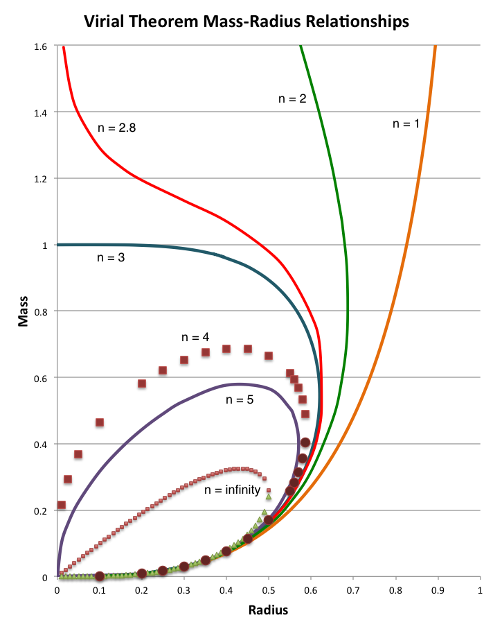
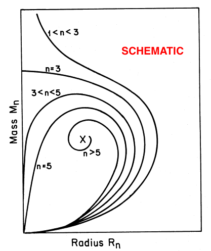
is plotted for seven different values of the polytropic index, <math>~n</math>, as indicated, in the lefthand diagram of the following composite figure. For comparison, the schematic diagram displayed on the righthand side of the figure is a reproduction of Figure 17 from Appendix B of Stahler (1983). It seems that our derived, analytically prescribable, mass-radius relationship — which is, in essence, a statement of the scalar virial theorem — embodies most of the attributes of the mass-radius relationship for pressure-truncated polytropes that were already understood, and conveyed schematically, by Stahler in 1983.
Let's do this again using the mass-radius relation as written explicitly in terms of the normalizations, <math>~M_\mathrm{SWS}</math> and <math>~R_\mathrm{SWS}</math>. The relevant, generic nonlinear equation is,
|
<math>~0</math> |
<math>~=</math> |
<math>~ \biggl( \frac{R}{R_\mathrm{SWS}} \biggr)^4 - \biggl( \frac{R}{R_\mathrm{SWS}} \biggr)^{(n-3)/n} \biggl[ \biggl(\frac{3}{4\pi} \biggr) \frac{M}{M_\mathrm{SWS}} \biggr]^{(n+1)/n} + \frac{3}{20\pi} \biggl( \frac{n+1}{n}\biggr) \biggl( \frac{M}{M_\mathrm{SWS}} \biggr)^2 \, . </math> |
Analytically determined roots:
- <math>~n=1</math>
<math>~\frac{M}{M_\mathrm{SWS}} = \biggl( \frac{10\pi}{3}\biggr)^{1 / 2} \biggl(\frac{R}{R_\mathrm{SWS}} \biggr)^3 \biggl[ \frac{3\cdot 5}{2^3\pi} - \biggl(\frac{R}{R_\mathrm{SWS}} \biggr)^2 \biggr]^{-1/2} </math> for, <math>~0 \le \frac{R}{R_\mathrm{SWS}} \le \biggl(\frac{3\cdot 5}{2^3\pi}\biggr)^{1/2} \, .</math>
- <math>~n=3</math>
<math>~\frac{R}{R_\mathrm{SWS}} = \biggl\{ \biggl[ \biggl(\frac{3}{4\pi}\biggr)\frac{M}{M_\mathrm{SWS}}\biggr]^{4/3} - \biggl(\frac{1}{5\pi}\biggr) \biggl( \frac{M}{M_\mathrm{SWS}}\biggr)^2 \biggr\}^{1/4} </math> for, <math>~0 \le \frac{M}{M_\mathrm{SWS}} \le \biggl(\frac{3^4\cdot 5^3}{2^8\pi}\biggr)^{1/2} \, .</math>
- Isothermal (explained immediately below)
<math>~\frac{M}{M_\mathrm{SWS}} = \frac{5}{2} \biggl( \frac{R}{R_\mathrm{SWS}} \biggr) \biggl\{ 1 \pm \biggl[ 1 - \frac{16\pi}{15}\biggl( \frac{R}{R_\mathrm{SWS}} \biggr)^2 \biggr]^{1 / 2} \biggr\} </math> for, <math>~0 \le \frac{R}{R_\mathrm{SWS}} \le \biggl(\frac{3\cdot 5}{2^4\pi}\biggr)^{1/2} \, .</math>
First, we'll create a table of the normalized coordinate values that satisfy this nonlinear expression.
| <math>~n =2</math> | <math>~n =2.8</math> | <math>~n =3.5</math> | <math>~n = 4</math> | <math>~n = 5</math> | |||||||||||||||||||||||||||||||||||||||||||||||||||||||||||||||||||||||||||||||||||||||||||||||||||||||||||||||||||||||||||||||||||||||||||||||||||||||||||||||||||||||||||||||||||||||||||||||||||||||||||||||||||||||||||||||||||||||||||||||||||||||||||||||||||||||||||||||||||||||||||||||||||||||||||||||||||||||||||||||||||||||||||||||||||||||||||||||||||||||||||||||||||||||||||||||||||||||||||||||||||||
|
|
|
|
|
|||||||||||||||||||||||||||||||||||||||||||||||||||||||||||||||||||||||||||||||||||||||||||||||||||||||||||||||||||||||||||||||||||||||||||||||||||||||||||||||||||||||||||||||||||||||||||||||||||||||||||||||||||||||||||||||||||||||||||||||||||||||||||||||||||||||||||||||||||||||||||||||||||||||||||||||||||||||||||||||||||||||||||||||||||||||||||||||||||||||||||||||||||||||||||||||||||||||||||||||||||||
From a free-energy analysis of isothermal spheres, we have demonstrated that, when the structural form factors are all set to unity, the statement of virial equilibrium is,
|
<math>~0</math> |
<math>~=</math> |
<math>~ \biggl( \frac{R}{R_\mathrm{SWS}} \biggr)^4 - \frac{3}{4\pi} \biggr( \frac{M}{M_\mathrm{SWS}} \biggr) \biggl( \frac{R}{R_\mathrm{SWS}} \biggr) + \frac{3}{20\pi} \biggl( \frac{M}{M_\mathrm{SWS}} \biggr)^2 \, , </math> |
where, in order to be consistent with the above polytropic normalizations, we have adopted the isothermal normalizations,
|
<math>~M_\mathrm{SWS}\biggr|_\mathrm{isothermal} \equiv \biggl( \frac{c_s^8}{G^3 P_e} \biggr)^{1 / 2} \, ,</math> |
and |
<math>~R_\mathrm{SWS}\biggr|_\mathrm{isothermal} \equiv \biggl( \frac{c_s^4}{G P_e} \biggr)^{1 / 2} \, .</math> |
This is a quadratic equation that can be readily solved to provide an analytic expression for the isothermal mass-radius relation; the relevant expression has already been provided, above.
Confirmation
Rewriting the just-derived virial theorem expression in terms of Stahler's dimensionless radius and mass variables, written in the abbreviated form,
|
<math>~\mathcal{X}</math> |
<math>~\equiv</math> |
<math>~\frac{R_\mathrm{eq}}{R_\mathrm{SWS}} \, ,</math> |
|
<math>~\mathcal{Y}</math> |
<math>~\equiv</math> |
<math>~\frac{M_\mathrm{limit}}{M_\mathrm{SWS}} \, ,</math> |
we have,
|
<math>~0</math> |
<math>~=</math> |
<math>~\biggl[ \mathcal{X} \cdot \frac{R_\mathrm{SWS}}{R_\mathrm{mod}} \biggr]^4 - \biggl[ \mathcal{X} \cdot \frac{R_\mathrm{SWS}}{R_\mathrm{mod}} \biggr]^{(n-3)/n} \biggl[ \mathcal{Y} \cdot \frac{M_\mathrm{SWS}}{M_\mathrm{mod}} \biggr]^{(n+1)/n} + \biggl[ \mathcal{Y} \cdot \frac{M_\mathrm{SWS}}{M_\mathrm{mod}} \biggr]^2</math> |
|
|
<math>~=</math> |
<math>~\mathcal{X}^4 \biggl\{ \biggl( \frac{4\pi}{3} \biggr)^{n/(n+1)} \biggl[ \frac{3(n+1)}{4\pi n} \biggr]^{1/2} \frac{\mathcal{A}_{M_\ell}^{1/2}}{\mathcal{B}_{M_\ell}^{n/(n+1)}} \biggr\}^4 + \mathcal{Y}^2 \biggl\{ \biggl( \frac{4\pi}{3} \biggr)^{2n/(n+1)} \biggl[ \frac{3(n+1)}{4\pi n} \biggr]^{3/2} \frac{\mathcal{A}_{M_\ell}^{3/2}}{\mathcal{B}_{M_\ell}^{2n/(n+1)}} \biggr\}^2</math> |
|
|
|
<math>~ - \mathcal{X}^{(n-3)/n} \mathcal{Y}^{(n+1)/n} \biggl\{ \biggl( \frac{4\pi}{3} \biggr)^{n/(n+1)} \biggl[ \frac{3(n+1)}{4\pi n} \biggr]^{1/2} \frac{\mathcal{A}_{M_\ell}^{1/2}}{\mathcal{B}_{M_\ell}^{n/(n+1)}}\biggr\}^{(n-3)/n} \biggl\{ \biggl( \frac{4\pi}{3} \biggr)^{2n/(n+1)} \biggl[ \frac{3(n+1)}{4\pi n} \biggr]^{3/2} \frac{\mathcal{A}_{M_\ell}^{3/2}}{\mathcal{B}_{M_\ell}^{2n/(n+1)}} \biggr\}^{(n+1)/n} </math> |
|
|
<math>~=</math> |
<math>~\mathcal{X}^4 \biggl\{ \biggl( \frac{4\pi}{3} \biggr)^{4n/(n+1)} \biggl[ \frac{3(n+1)}{4\pi n} \biggr]^{2} \frac{\mathcal{A}_{M_\ell}^{2}}{\mathcal{B}_{M_\ell}^{4n/(n+1)}} \biggr\} + \mathcal{Y}^2 \biggl\{ \biggl( \frac{4\pi}{3} \biggr)^{4n/(n+1)} \biggl[ \frac{3(n+1)}{4\pi n} \biggr]^{3} \frac{\mathcal{A}_{M_\ell}^{3}}{\mathcal{B}_{M_\ell}^{4n/(n+1)}} \biggr\}</math> |
|
|
|
<math>~ - \mathcal{X}^{(n-3)/n} \mathcal{Y}^{(n+1)/n} \biggl\{ \biggl( \frac{4\pi}{3} \biggr)^{[(n-3)+2(n+1)]/(n+1)} \biggl[ \frac{3(n+1)}{4\pi n} \biggr]^{[(n-3)+3(n+1)]/2n} \frac{\mathcal{A}_{M_\ell}^{[(n-3)+3(n+1)]/2n}}{\mathcal{B}_{M_\ell}^{[(n-3)+2(n+1)]/(n+1)}}\biggr\} </math> |
|
|
<math>~=</math> |
<math>~\biggl\{\mathcal{X}^4 + \biggl[\frac{3(n+1)}{4\pi n}\biggr] \mathcal{A}_{M_\ell} \mathcal{Y}^2 \biggr\} \biggl\{ \biggl( \frac{4\pi}{3} \biggr)^{4n/(n+1)} \biggl[ \frac{3(n+1)}{4\pi n} \biggr]^{2} \frac{\mathcal{A}_{M_\ell}^{2}}{\mathcal{B}_{M_\ell}^{4n/(n+1)}} \biggr\}</math> |
|
|
|
<math>~ - \mathcal{X}^{(n-3)/n} \mathcal{Y}^{(n+1)/n} \biggl\{ \biggl( \frac{4\pi}{3} \biggr)^{(3n-1)/(n+1)} \biggl[ \frac{3(n+1)}{4\pi n} \biggr]^{2} \frac{\mathcal{A}_{M_\ell}^{2}}{\mathcal{B}_{M_\ell}^{(3n-1)/(n+1)}}\biggr\} </math> |
|
|
<math>~=</math> |
<math>~ \biggl[ \biggl(\frac{4\pi}{3}\biggr) \mathcal{X}^4 - \mathcal{B}_{M_\ell} \cdot \mathcal{X}^{(n-3)/n} \mathcal{Y}^{(n+1)/n} + \biggl(\frac{n+1}{n}\biggr) \mathcal{A}_{M_\ell} \mathcal{Y}^2 \biggr] \biggl\{ \biggl( \frac{4\pi}{3} \biggr)^{(3n-1)/(n+1)} \biggl[ \frac{3(n+1)}{4\pi n} \biggr]^{2} \frac{\mathcal{A}_{M_\ell}^{2}}{\mathcal{B}_{M_\ell}^{4n/(n+1)}} \biggr\} \, . </math> |
Replacing <math>~\mathcal{A}_{M_\ell}</math> and <math>~\mathcal{B}_{M_\ell}</math> with <math>~\mathcal{A}</math> and <math>~\mathcal{B}</math>, as prescribed by their defined relationships, the expression inside the square brackets becomes the above, boxed-in mass-radius relationship, namely,
|
<math>~ \frac{4\pi}{3} \cdot \mathcal{X}^4 - \mathcal{B} \cdot \mathcal{X}^{(n-3)/n} \biggl[ \mathcal{Y} \biggl( \frac{M_\mathrm{tot}}{M_\mathrm{limit}} \biggr) \biggr]^{(n+1)/n} +~ \mathcal{A} \biggl( \frac{n+1}{n} \biggr) \biggl[ \mathcal{Y} \biggl( \frac{M_\mathrm{tot}}{M_\mathrm{limit}} \biggr) \biggr]^{2} </math> |
<math>~=</math> |
<math>~0 \, .</math> |
In Terms of Structural Form-Factors
Alternatively, replacing <math>~\mathcal{A}_{M_\ell}</math> and <math>~\mathcal{B}_{M_\ell}</math> by their expressions in terms of the structural form factors gives,
|
<math>~ \frac{4\pi}{3} \cdot \mathcal{X}^4 - \mathcal{X}^{(n-3)/n} \mathcal{Y}^{(n+1)/n} \biggl( \frac{4\pi}{3} \biggr)^{-1/n} \frac{\tilde\mathfrak{f}_A}{\tilde\mathfrak{f}_M^{(n+1)/n}} + \mathcal{Y}^2\biggl( \frac{n+1}{5n} \biggr) \frac{\tilde\mathfrak{f}_W }{\tilde\mathfrak{f}_M^2} </math> |
<math>~=</math> |
<math>~0 \, .</math> |
Finally, inserting into this relation the expressions presented above for the structural form-factors, <math>~\tilde\mathfrak{f}_M</math> and <math>~\tilde\mathfrak{f}_A</math>, namely,
|
<math>~\tilde\mathfrak{f}_M</math> |
<math>~=</math> |
<math>~ \biggl[ - \frac{3\Theta^'}{\xi} \biggr]_{\tilde\xi} </math> |
|
<math>~ \tilde\mathfrak{f}_A </math> |
<math>~=</math> |
<math>~ \tilde\theta^{n+1} + \biggl[ \frac{(n+1)}{3\cdot 5} \biggr] \tilde\xi^2 \cdot \tilde\mathfrak{f}_W </math> |
gives us the desired,
|
Virial Theorem written in terms of <math>~\mathcal{X}</math>, <math>~\mathcal{Y}</math>, and <math>~\tilde\mathfrak{f}_W</math> <math>~ 4\pi \cdot \mathcal{X}^4 ~- ~ \mathcal{X}^{(n-3)/n} \mathcal{Y}^{(n+1)/n} ( 4\pi)^{-1/n} \biggl[\frac{\tilde\xi}{(-\tilde\theta^')}\biggr]^{(n+1)/n} \biggl[\tilde\theta^{n+1} + \frac{(n+1)\tilde\xi^2}{3\cdot 5} \cdot \tilde\mathfrak{f}_W \biggr] ~+ ~ \mathcal{Y}^2\biggl( \frac{n+1}{3\cdot 5n} \biggr) \frac{\tilde\xi^2}{(- \tilde\theta^')^2} \cdot \tilde\mathfrak{f}_W = 0 \, . </math> |
Relating and Reconciling Two Mass-Radius Relationships for n = 5 Polytropes
Now, let's examine the case of pressure-truncated, <math>~n=5</math> polytropes. As we have discussed in the context of detailed force-balanced models, Stahler (1983) has deduced that all <math>~n=5</math> equilibrium configurations obey the mass-radius relationship,
|
<math>~\biggl( \frac{M_\mathrm{limit}}{M_\mathrm{SWS}} \biggr)^2 - 5 \biggl( \frac{M_\mathrm{limit}}{M_\mathrm{SWS}} \biggr)\biggl( \frac{R_\mathrm{eq}}{R_\mathrm{SWS}} \biggr) + \frac{2^2 \cdot 5 \pi}{3} \biggl( \frac{R_\mathrm{eq}}{R_\mathrm{SWS}} \biggr)^4 </math> |
<math>~=</math> |
<math>~0 \, ,</math> |
where, as reviewed above, the mass and radius normalizations, <math>~M_\mathrm{SWS}</math> and <math>~R_\mathrm{SWS}</math>, may be treated as constants once the parameters <math>~K</math> and <math>~P_e</math> are specified. In contrast to this, the mass-radius relationship that we have just derived from the virial theorem for pressure-truncated, <math>~n=5</math> polytropes is,
<math> \biggl( \frac{M_\mathrm{limit}}{M_\mathrm{mod}} \biggr)^2 - \biggl( \frac{R_\mathrm{eq}}{R_\mathrm{mod}} \biggr)^{2/5} \biggl( \frac{M_\mathrm{limit}}{M_\mathrm{mod}} \biggr)^{6/5} + \biggl( \frac{R_\mathrm{eq}}{R_\mathrm{mod}} \biggr)^4 = 0 \, , </math>
where the mass and radius normalizations,
|
<math>~M_\mathrm{mod}\biggr|_{n=5}</math> |
<math>~=</math> |
<math>~M_\mathrm{SWS} \biggl( \frac{3\mathcal{B}_{M_\ell}}{4\pi} \biggr)^{5/3} \biggl[ \frac{2\cdot 5\pi}{3^2 \mathcal{A}_{M_\ell}} \biggr]^{3/2} \, ,</math> |
|
<math>~R_\mathrm{mod}\biggr|_{n=5}</math> |
<math>~=</math> |
<math>~R_\mathrm{SWS} \biggl( \frac{3\mathcal{B}_{M_\ell}}{4\pi}\biggr)^{5/6} \biggl[ \frac{2\cdot 5\pi}{3^2\mathcal{A}_{M_\ell}} \biggr]^{1/2} \, ,</math> |
depend, not only on <math>~K</math> and <math>~P_e</math> via the definitions of <math>~M_\mathrm{SWS}</math> and <math>~R_\mathrm{SWS}</math>, but also on the structural form factors via the free-energy coefficients, <math>~\mathcal{A}_{M_\ell}</math> and <math>~\mathcal{B}_{M_\ell}</math>. While these two separate mass-radius relationships are similar, they are not identical. In particular, the middle term involving the cross-product of the mass and radius contains different exponents in the two expressions. It is not immediately obvious how the two different polynomial expressions can be used to describe the same physical sequence.
This apparent discrepancy is reconciled as follows: The structural form factors — and, hence, the free-energy coefficients — vary from equilibrium configuration to equilibrium configuration. So it does not make sense to discuss evolution along the sequence that is defined by the second of the two polynomial expressions. If you want to know how a given system's equilibrium radius will change as its mass changes, the first of the two polynomials will do the trick. However, the equilibrium radius of a given system can be found by looking for extrema in the free-energy function while holding the free-energy coefficients, <math>~\mathcal{A}_{M_\ell}</math> and <math>~\mathcal{B}_{M_\ell}</math>, constant; more importantly, the relative stability of a given equilibrium system can be determined by analyzing the behavior of the system's free energy while holding the free-energy coefficients constant. Dynamically stable versus dynamically unstable configurations can be readily distinguished from one another along the sequence that is defined by the second polynomial expression; they cannot be readily distinguished from one another along the sequence that is defined by the first polynomial expression. It is useful, therefore, to determine how to map a configuration's position on one of the sequences to the other.
Plotting Stahler's Relation
Switching, again, to the shorthand notation,|
<math>~\mathcal{X}</math> |
<math>~\equiv</math> |
<math>~\frac{R_\mathrm{eq}}{R_\mathrm{SWS}} \, ,</math> |
|
<math>~\mathcal{Y}</math> |
<math>~\equiv</math> |
<math>~\frac{M_\mathrm{tot}}{M_\mathrm{SWS}} \, ,</math> |
the equilibrium mass-radius relation defined by the first of the two polynomial expressions can be plotted straightforwardly in either of two ways.
Quadratic Equation
One way is to recognize that the polynomial is a quadratic equation whose solution is,
|
<math>~\mathcal{Y}_\pm</math> |
<math>~=</math> |
<math>~\frac{5}{2} \mathcal{X} \biggl\{ 1 \pm \biggl[ 1 - \biggl( \frac{2^4\cdot \pi}{3\cdot 5} \biggr) \mathcal{X}^2 \biggr]^{1/2} \biggr\} \, .</math> |
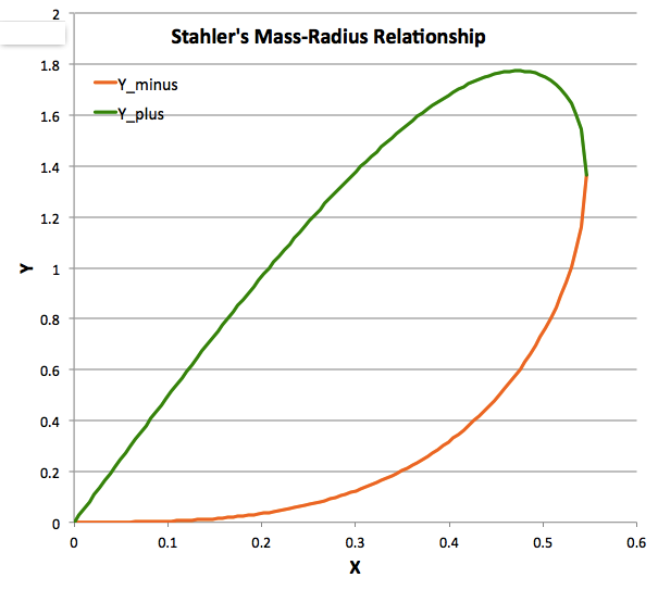
In the figure shown here on the right — see also the bottom panel of Figure 2 in our accompanying discussion of detailed force-balance models — Stahler's mass-radius relation has been plotted using the solution to this quadratic equation; the green segment of the displayed curve was derived from the positive root while the segment derived from the negative root is shown in orange. The two curve segments meet at the maximum value of the normalized equilibrium radius, namely, at
<math>\mathcal{X}_\mathrm{max} \equiv \biggl[ \frac{3\cdot 5}{2^4 \pi} \biggr]^{1/2} \approx 0.54627 \, .</math>
We note that, when <math>~\mathcal{X} = \mathcal{X}_\mathrm{max}</math>, <math>~\mathcal{Y} = (5\mathcal{X}_\mathrm{max}/2) \approx 1.36569</math>. Along the entire sequence, the maximum value of <math>~\mathcal{Y}</math> occurs at the location where <math>~d\mathcal{Y}/d\mathcal{X} = 0</math> along the segment of the curve corresponding to the positive root. This occurs along the upper segment of the curve where <math>~\mathcal{X}/\mathcal{X}_\mathrm{max} = \sqrt{3}/2</math>, at the location,
<math>\mathcal{Y}_\mathrm{max} \equiv \biggl[ \frac{3^3 \cdot 5^2}{2^6 } \biggr]^{1/2} \mathcal{X}_\mathrm{max} = \biggl[ \frac{3^4 \cdot 5^3}{2^{10} \pi } \biggr]^{1/2} \approx 1.77408 \, .</math>
Parametric Relations
The other way is to determine the normalized mass and normalized radius individually through Stahler's pair of parametric relations. Drawing partly from our above discussion and partly from a separate discussion where we provide a tabular summary of the properties of pressure-truncated <math>~n=5</math> polytropes, these are,
|
<math> ~\mathcal{X}\biggr|_{n=5} </math> |
<math>~=~</math> |
<math> \biggl( \frac{5}{4\pi} \biggr)^{1/2} \tilde\xi \tilde\theta^{2} = \biggl\{ \frac{3\cdot 5}{2^2 \pi} \biggl[ \frac{\tilde\xi^2/3}{(1+\tilde\xi^2/3)^{2}} \biggr] \biggr\}^{1/2} \, , </math> |
|
<math> ~\mathcal{Y}\biggr|_{n=5} </math> |
<math>~=~</math> |
<math> \biggl( \frac{5^3}{4\pi} \biggr)^{1/2} \tilde\theta (- \tilde\xi^2 \tilde\theta^') = \biggl[ \biggl( \frac{3 \cdot 5^3}{2^2\pi} \biggr) \frac{(\tilde\xi^2/3)^3}{(1+\tilde\xi^2/3)^{4}} \biggr]^{1/2} \, . </math> |
The entire sequence will be traversed by varying the Lane-Emden parameter, <math>~\tilde\xi</math>, from zero to infinity. Using the first of these two expressions, we have determined, for example, that the point along the sequence corresponding to the maximum normalized equilibrium radius, <math>~\mathcal{X}_\mathrm{max}</math>, is associated with an embedded <math>~n=5</math> polytrope whose truncated, dimensionless Lane-Emden radius is,
<math> ~\tilde\xi \biggr|_{\mathcal{X}_\mathrm{max}} = 3^{1/2} \, . </math>
Similarly, we have determined that the point along the sequence that corresponds to the maximum dimensionless mass, <math>~\mathcal{Y}_\mathrm{max}</math>, is associated with an embedded <math>~n=5</math> polytrope whose truncated, dimensionless Lane-Emden radius is, precisely,
<math> ~\tilde\xi \biggr|_{\mathcal{Y}_\mathrm{max}} = 3 \, . </math>
|
Referring back to our review of turning points along equilibrium sequences and, especially, the work of Kimura (1981b), we appreciate that the point that corresponds to the maximum mass, <math>~\mathcal{Y}_\mathrm{max}</math>, is the turning point that Kimura refers to as the "extremum in M1" along a p1 sequence. As we have highlighted, according to Kimura, this point should occur along the sequence where <math>~h_G=0</math>, that is, where the following condition applies: <math>~\frac{\tilde\theta^{n+1}}{(\tilde\theta^')^2} = \frac{(n-3)}{2} \, .</math> For the specific case being studied here, namely, <math>~n = 5</math> polytropic configurations, we therefore expect from Kimura's work that <math>~[\tilde\theta^6/(\tilde\theta^')^2] = 1</math> at the "maximum mass" turning point. Given that, <math>~\tilde\xi \biggr|_{\mathcal{Y}_\mathrm{max}} = 3</math> <math>~\Rightarrow</math> <math>\tilde\theta_{n=5} = \frac{1}{2}</math> and <math>\tilde\theta_{n=5}^' = -\frac{1}{8} \, ,</math> we see that Kimura's condition holds and, hence, that our identification of the location along the sequence of the maximum mass matches Kimura's identification of the location of that turning point. We appreciate, as well, that the point corresponding to the maximum normalized equilibrium radius, <math>~\mathcal{X}_\mathrm{max}</math>, is the turning point that Kimura would reference as the "extremum in r1" along a p1 sequence. Following Kimura's analysis we have shown that this point occurs along the sequence where the following condition applies: <math>~\frac{\xi (-\theta^')}{\tilde\theta} = \frac{2}{(n-1)} \, ,</math> that is, for the specific case being studied here, we should expect <math>~[\tilde\xi (-\tilde\theta^')/\tilde\theta] = 1/2</math> at the "maximum radius" turning point. Given that, <math>~\tilde\xi \biggr|_{\mathcal{X}_\mathrm{max}} = 3^{1/2}</math> <math>~\Rightarrow</math> <math>\tilde\theta_{n=5} = 2^{-1/2}</math> and <math>\tilde\theta_{n=5}^' = -(2^3 \cdot 3)^{-1/2} \, ,</math> we see that Kimura's condition holds and, hence, that our identification of the location along the sequence of the maximum radius matches Kimura's identification of the location of that turning point. |
Discussion
Notice that if the quadratic equation is used to map out the mass-radius relationship, the parameter, <math>~\tilde\xi</math>, never explicitly enters the discussion. Instead, a radius <math>~0 \le \mathcal{X} \le \mathcal{X}_\mathrm{max}</math> is specified and the two equilibrium masses associated with <math>~\mathcal{X}</math> — call them, <math>~\mathcal{Y}_+</math> and <math>~\mathcal{Y}_-</math> — are determined. (The values of the two masses are degenerate at both limiting values of <math>~\mathcal{X}</math>.) If the pair of parametric relations is used, instead, only one value of the mass is obtained for each specified value of <math>~\tilde\xi</math>. As <math>~\tilde\xi</math> is increased from <math>~0</math> to <math>~\sqrt{3}</math>, <math>~\mathcal{X}</math> increases monotonically from <math>~0</math> to <math>~\mathcal{X}_\mathrm{max}</math> and the corresponding mass is (only) <math>~\mathcal{Y}_-</math>; that is, as <math>~\tilde\xi</math> is increased from <math>~0</math> to <math>~\sqrt{3}</math>, we move away from the origin in a counter-clockwise direction along the lower segment (colored orange in the above figure) of the plotted equlibrium sequence. Then, as <math>~\tilde\xi</math> is increased from <math>~\sqrt{3}</math> to <math>~\infty</math>, we continue to move in a counter-clockwise direction along the equilibrium sequence, but now along the upper segment (colored green in the above figure) of the sequence, back to the origin; that is to say, <math>~\mathcal{X}</math> steadily decreases from <math>~\mathcal{X}_\mathrm{max}</math> back to <math>~0</math> and this time the relevant associated mass is the positive root of the quadratic relation, <math>~\mathcal{Y}_+</math>.
Clearly, then, each value of <math>~\mathcal{X}</math> is associated with two different values of the parametric parameter, <math>~\tilde\xi</math>. By inverting the <math>~\mathcal{X}(\tilde\xi)</math> parametric expression we see that, the two values of <math>~\tilde\xi</math> associated with a given equilibrium radius are,
|
<math>~\tilde\xi_\pm</math> |
<math>~=</math> |
<math>~\biggl\{\frac{3}{\alpha} \biggl[ 1 \pm \sqrt{1 - \alpha^2} \biggr] \biggr\}^{1/2} \, ,</math> |
where,
|
<math>~\alpha</math> |
<math>~\equiv</math> |
<math>~\frac{(\mathcal{X}/\mathcal{X}_\mathrm{xmax})^2}{2-(\mathcal{X}/\mathcal{X}_\mathrm{xmax})^2} \, .</math> |
We note as well that, for a given equilibrium radius, <math>~\mathcal{X}</math>, the ratio of the two mass solutions is given by a very simple expression, namely,
|
<math>~\frac{\mathcal{Y}_-}{\mathcal{Y}_+} = \frac{\tilde\xi_-^2}{3}</math> |
or |
<math>~\frac{\mathcal{Y}_+}{\mathcal{Y}_-} = \frac{\tilde\xi_+^2}{3} \, .</math> |
This implies, as well, that,
|
<math>~\tilde\xi_+ \cdot \tilde\xi_-</math> |
<math>~=</math> |
<math>~3\, .</math> |
Plotting the Virial Theorem Relation
Drawing from our above derivations, the concise free-energy expression that reflects the properties of pressure-truncated <math>~n = 5</math> polytropic configurations is,
|
<math>~\mathfrak{G}^*</math> |
<math>~=</math> |
<math>~ - \frac{18}{5}\cdot \mathcal{A}_{M_\ell} \biggl( \frac{M_\mathrm{limit}}{M_\mathrm{SWS}} \biggr)^{2} \biggl(\frac{R}{R_\mathrm{SWS}}\biggr)^{-1} +~ 5\mathcal{B}_{M_\ell} \cdot \biggl( \frac{M_\mathrm{limit}}{M_\mathrm{SWS}} \biggr)^{6/5} \biggl(\frac{R}{R_\mathrm{SWS}}\biggr)^{-3/5} +~ \frac{4\pi}{3} \cdot \biggl(\frac{R}{R_\mathrm{SWS}}\biggr)^{3} \, , </math> |
where,
|
<math>~\mathcal{A}_{M_\ell}</math> |
<math>~=</math> |
<math>~ \frac{1}{5} \cdot \frac{\tilde\mathfrak{f}_W}{\tilde\mathfrak{f}_M^2} =\frac{1}{3^2\cdot 5} \biggl( \frac{\tilde\xi}{-\tilde\theta^'} \biggr)^2 \tilde\mathfrak{f}_W \, , </math> |
|
<math>~\mathcal{B}_{M_\ell}</math> |
<math>~=</math> |
<math>~ \biggl( \frac{3}{4\pi}\biggr)^{1/5} \frac{\tilde\mathfrak{f}_A}{\tilde\mathfrak{f}_M^{6/5}} = \frac{1}{3}( 4\pi)^{-1/5} \biggl( \frac{\tilde\xi}{-\tilde\theta^'} \biggr)^{6/5} \biggl[ \tilde\theta^6 + \frac{2}{5} \cdot \tilde\xi^2 \tilde\mathfrak{f}_W \biggr] \, . </math> |
The virial theorem which is derived from this free-energy expression provides a mass-radius relationship to be compared with the detailed force-balance relationship presented by Stahler. Because our intent is to make this comparison, we begin with the virial theorem as written in terms of the variables, <math>~\mathcal{X}</math> and <math>~\mathcal{Y}</math>, and specialized for the case of <math>~n = 5</math> polytropic configurations. Written in terms of the (constant) coefficients in the free-energy expression, we have
|
<math>~ \mathcal{X}^4 - \frac{3\mathcal{B}_{M_\ell}}{4\pi} \cdot ( \mathcal{X} \mathcal{Y}^3 )^{2/5} +~ \frac{9 \mathcal{A}_{M_\ell}}{10\pi}\cdot \mathcal{Y}^{2} </math> |
<math>~=</math> |
<math>~0 \, ;</math> |
or, from above, the
|
Virial Theorem written in terms of <math>~\mathcal{X}</math>, <math>~\mathcal{Y}</math>, and <math>~\tilde\mathfrak{f}_W</math> <math>~ \mathcal{X}^4 ~- ~ (\mathcal{X} \mathcal{Y}^3)^{2/5} \biggl[\frac{\tilde\xi}{4\pi (-\tilde\theta^')}\biggr]^{6/5} \biggl[\tilde\theta^{6} + \frac{2}{5} \cdot \tilde\xi^2 \tilde\mathfrak{f}_W \biggr] ~+ ~ \mathcal{Y}^2 \biggl[\frac{\tilde\xi}{(- \tilde\theta^')} \biggr]^2 \frac{\tilde\mathfrak{f}_W}{2\cdot 5^2 \pi} = 0 \, , </math> |
where, specifically for <math>~n = 5</math> polytropic configurations — see our summary of the radial profiles of physical variables and our determination of expressions for the structural form-factors,
|
<math>~\tilde\theta</math> |
<math>~=</math> |
<math>~ ( 1+ \ell^2 )^{-1/2} \, , </math> |
|
<math>~\tilde\theta^'</math> |
<math>~=</math> |
<math>~ - 3^{-1/2} \ell ( 1+ \ell^2 )^{-3/2} \, , </math> |
|
<math>~\mathfrak{f}_W</math> |
<math>~=</math> |
<math>~ \frac{5}{2^4} \cdot \ell^{-5} \biggl[ \ell \biggl( \ell^4 - \frac{8}{3}\ell^2 - 1 \biggr)(1 + \ell^2)^{-3} + \tan^{-1}(\ell ) \biggr] \, , </math> |
|
<math>~\ell^2</math> |
<math>~\equiv</math> |
<math>~ \frac{\tilde\xi^2}{3} \, . </math> |
Once numerical values have been assigned to the free-energy coefficients, <math>~\mathcal{A}_{M_\ell}</math> and <math>~\mathcal{B}_{M_\ell}</math>, the mass-radius relationship given by the scalar virial theorem can be compared quantitatively with Stahler's (detailed force-balance) mass-radius relationship. The simplest, physically reasonable approximation would be to assume uniform-density structures, in which case, <math>~\tilde\mathfrak{f}_M = \tilde\mathfrak{f}_W = \tilde\mathfrak{f}_A = 1</math>, and accordingly, <math>~\mathcal{A}_{M_\ell} = 5^{-1}</math> and <math>~\mathcal{B}_{M_\ell} = (4\pi/3)^{-1/5}</math>. But a better approximation would be to assign values to the structural form-factors that properly represent the properties of at least one detailed force-balanced model. By way of illustration, the following table details what the proper values are for the two free-energy coefficients, and other relevant parameters, specifically for the model along Stahler's sequence that sits at <math>~\mathcal{Y}_\mathrm{max}</math> — that is, the model whose truncation radius is <math>~\tilde\xi = 3</math>. As is recorded in the table, in this case the precise values of the free-energy coefficients are,
|
<math>~\mathcal{A}_{M_\ell}</math> |
<math>~=</math> |
<math>~ \biggl( \frac{2^4 \pi^2}{3^7} \biggr)^{1/2} \, , </math> |
|
<math>~\mathcal{B}_{M_\ell}</math> |
<math>~=</math> |
<math>~ \biggl( \frac{3}{2^{14}\pi} \biggr)^{1/5} \biggl[ 1 + \biggl( \frac{2^6\pi^2}{3^3} \biggr)^{1/2}\biggr] \, . </math> |
Notice that, by choosing <math>~\tilde\xi = 3</math>, the evaluation of <math>~\tilde\mathfrak{f}_W</math> is particularly simple, in part, because <math>~\tan^{-1}(\ell) = \tan^{-1} \sqrt{3} = \pi/3</math>, but also because the term <math>~(\ell^4 - 8\ell^2/3 - 1)</math> equals zero.
|
Determination of Coefficient Values in the Specific Case of <math>~\tilde\xi = 3</math> |
||
|---|---|---|
|
Quantity |
Analytic Evaluation |
Numerical |
|
<math>~\ell</math> |
<math>~3^{1/2}</math> |
<math>~1.732051</math> |
|
<math>~\tilde\theta</math> |
<math>~2^{-1}</math> |
<math>~0.5</math> |
|
<math>~\tilde\theta^'</math> |
<math>~2^{-3}</math> |
<math>~0.125</math> |
|
<math>~\mathcal{X}</math> |
<math>~\biggl( \frac{3^2\cdot 5}{2^6\pi} \biggr)^{1/2}</math> |
<math>~0.473087</math> |
|
<math>~\mathcal{Y}</math> |
<math>~\biggl( \frac{3^4\cdot 5^3}{2^{10}\pi} \biggr)^{1/2}</math> |
<math>~1.774078</math> |
|
<math>~\tilde\mathfrak{f}_W</math> |
<math>~\biggl( \frac{5^2 \pi^2}{2^8\cdot 3^7} \biggr)^{1/2}</math> |
<math>~0.020993</math> |
|
<math>~\mathcal{A}_{M_\ell}</math> |
<math>~\biggl( \frac{2^4 \pi^2}{3^7} \biggr)^{1/2}</math> |
<math>~0.268711</math> |
|
<math>~\mathcal{B}_{M_\ell}</math> |
<math>~\biggl( \frac{3}{2^{14}\pi} \biggr)^{1/5} \biggl[ 1 + \biggl( \frac{2^6\pi^2}{3^3} \biggr)^{1/2}\biggr]</math> |
<math>~0.830395</math> |
|
<math>~G^*</math> |
<math>~\biggl( \frac{3\cdot 5^3}{2^{12}\pi} \biggr)^{1/2} [ 2^3\pi + 3^{5/2} ]</math> |
<math>~6.951544</math> |
|
Virial: <math>~\mathcal{X}^4 - \frac{3\mathcal{B}_{M_\ell}}{4\pi} \cdot (\mathcal{X}\mathcal{Y}^3 )^{2/5}</math> <math>~~~~~~~~~~+\frac{9 \mathcal{A}_{M_\ell}}{10\pi} \cdot \mathcal{Y}^2</math> |
<math>~ \frac{3^4\cdot 5^2}{2^{12}\pi} - \frac{3^4\cdot 5^2}{2^{12}\pi} \biggl[ 1 + \biggl( \frac{2^6\pi^2}{3^3} \biggr)^{1/2}\biggr]</math> <math>~~~~~~~~~~+ \biggl( \frac{3^5\cdot 5^4}{2^{18} \pi^2} \biggr)^{1/2} </math> |
Sums to zero, exactly! |
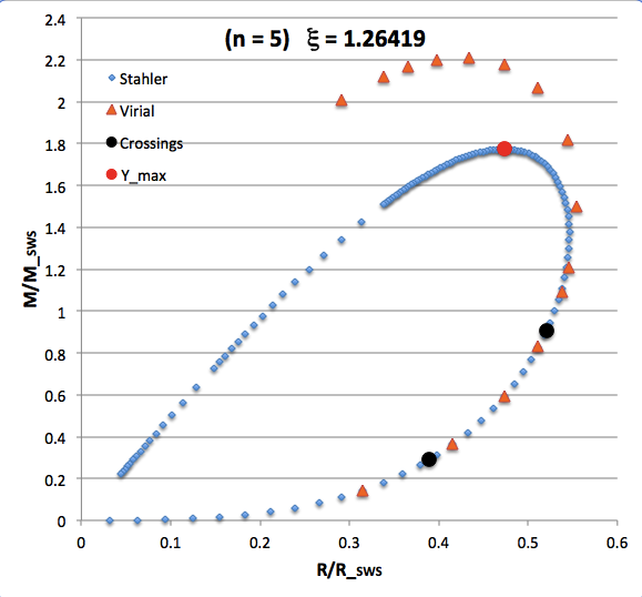
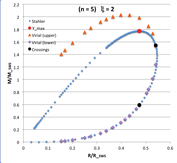
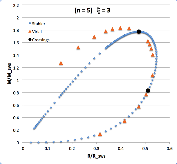
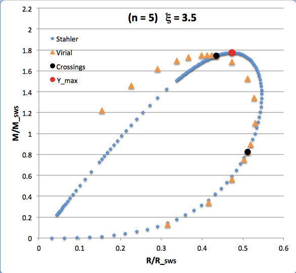
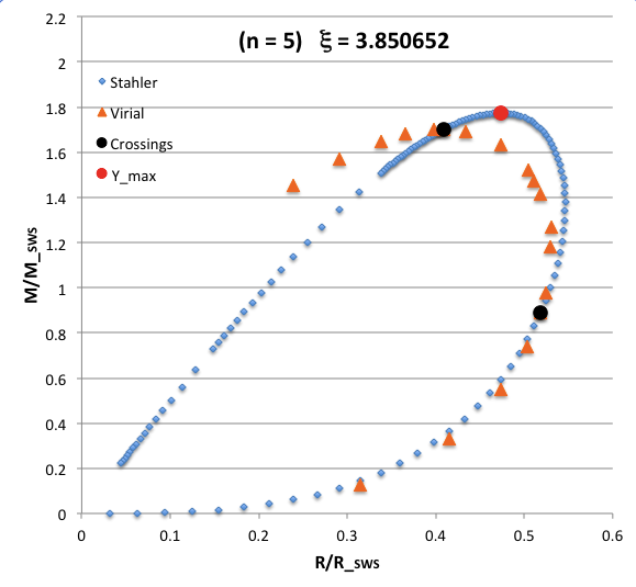
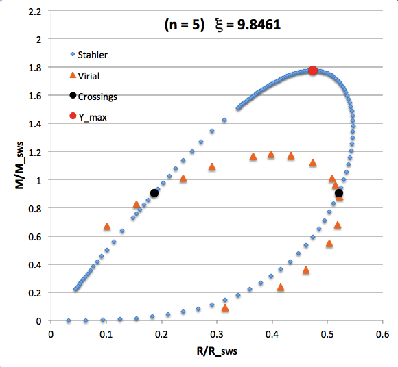
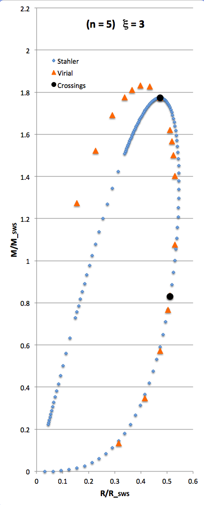
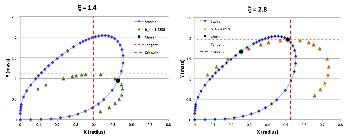
The curve traced out by the light-blue diamonds in each panel of the following comparison figure displays Stahler's analytically prescribed mass-radius relation; this curve is identical in all six panels and is the same as the curve displayed above in connection with our description of Stahler's mass-radius relation. Each point along this "Stahler" curve identifies a model having a different truncation radius, <math>~\tilde\xi</math>; as plotted here, starting near the origin and moving counter-clockwise around the curve, <math>~\tilde\xi</math> is varied from 0.05 to 42.5. As foreshadowed by the above discussion, the model having the greatest mass <math>~(\mathcal{Y}_\mathrm{max})</math> along the Stahler sequence — highlighted by the red filled circle in most of the figure panels — is defined by <math>~\tilde\xi = 3</math>.
In each figure panel, the curve traced out by the orange triangles — or, in one case, the orange triangles & light purple diamonds — displays the mass-radius relation defined by the virial theorem. These "Virial" curves are all defined by the same virial theorem polynomial expression, as just presented, but the coefficient of the <math>~\mathcal{Y}^2</math> term and the coefficient of the <math>~(\mathcal{X}\mathcal{Y}^3)^{2/5}</math> cross term — essentially, the value of <math>~\mathcal{A}_{M_\ell}</math> and the value of <math>~\mathcal{B}_{M_\ell}</math>, respectively — have different values in the six separate figure panels. In each case, a value has been specified for the parameter, <math>~\tilde\xi</math> (as identified in the title of each figure panel), and this, in turn, has determined the values of the two (constant) free-energy coefficients. For example, in the top-right figure panel whose title indicates <math>~\tilde\xi = 3</math>, the "Virial" curve traces the mass-radius relation prescribed by the virial theorem after the values of the free-energy coefficients have been set to values that correspond to a detailed force-balanced model with this specified truncation radius, that is (see the above table), <math>~\mathcal{A}_{M_\ell} = 0.268711</math> and <math>~\mathcal{B}_{M_\ell} = 0.830395</math>. Columns 2 and 3, respectively, of the table affixed to the bottom of the following comparison figure list the values of <math>~\mathcal{A}_{M_\ell}</math> and <math>~\mathcal{B}_{M_\ell}</math> that have been used to define the "Virial" curve in each of the six figure panels, in accordance with the value of <math>~\tilde\xi</math> listed in column 1 of the table.
|
Comparing Two Separate Mass-Radius Relations for Pressure-Truncated n = 5 Polytropes |
||||||
|---|---|---|---|---|---|---|
|
<math>~\tilde\xi</math> |
Free-Energy Coefficients |
Primary Overlap |
Secondary Overlap |
|||
|
<math>~\mathcal{A}_{M_\ell}</math> |
<math>~\mathcal{B}_{M_\ell}</math> |
<math>~\mathcal{X} \equiv \frac{R_\mathrm{eq}}{R_\mathrm{SWS}}</math> |
<math>~\mathcal{Y} \equiv \frac{M_\mathrm{limit}}{M_\mathrm{SWS}}</math> |
<math>~\mathcal{X}</math> |
<math>~\mathcal{Y}</math> |
|
|
1.26419 |
0.214429 |
0.758099 |
0.520269 |
0.904142 |
0.388938 |
0.289568 |
|
2 |
0.233842 |
0.779836 |
0.540671 |
1.544775 |
0.468918 |
0.570916 |
|
0.268711 |
0.830395 |
0.473087 |
1.774078 |
0.507387 |
0.798441 |
|
|
3.5 |
0.288708 |
0.861503 |
0.434310 |
1.744359 |
0.515168 |
0.859518 |
|
3.850652 |
0.303490 |
0.884746 |
0.408738 |
1.699778 |
0.518588 |
0.888969 |
|
9.8461 |
0.601012 |
1.313904 |
0.186424 |
0.904141 |
0.520269 |
0.904143 |
As is discussed more fully, below, in each of the six panels of the above comparison figure, the "Virial" curve intersects the "Stahler" curve at two locations. These points of intersection are identified by the black filled circles in each figure panel. In each case, the intersection point that is farthest along on the Stahler sequence — as determined by starting at the origin and moving counter-clockwise along the sequence — identifies the "Primary Overlap" between the two curves. That is to say, the <math>~(\mathcal{X}, \mathcal{Y})</math> coordinates of this point (see columns 4 and 5 of the table affixed to the bottom of the figure) are the coordinate values that are obtained by plugging the specified value of <math>~\tilde\xi</math> (see the title of the figure panel or column 1 of the affixed table) into Stahler's pair of parametric relations. The second point of intersection in each panel — which we will refer to as the "Secondary Overlap" points and whose coordinates are provided in columns 6 and 7 of the affixed table — appears to be fortuitous and of no particularly significant astrophysical interest.
The mass-radius diagram displayed in the top-right panel of the above comparison figure has been reproduced in the upper-left panel of the following figure — in this case, with a coordinate aspect ratio that is closer to 1:1 — along with color images of the corresponding free-energy surface, viewed from two different perspectives, and a three-column table listing the 3D coordinates, <math>~(X,Y,Z) = (R_\mathrm{eq}/R_\mathrm{SWS}, M_\mathrm{limit}/M_\mathrm{SWS}, \mathfrak{G}^*)</math>, of the seventeen points that have been used to define the displayed "Virial" curve. To be more explicit, the rainbow-colored free-energy surface, <math>~\mathfrak{G}^*(R,M_\mathrm{limit})</math>, has been defined by the free-energy function appropriate to pressure-truncated <math>~n=5</math> polytropic configurations as defined above, that is,
|
<math>~\mathfrak{G}^*</math> |
<math>~=</math> |
<math>~ - \frac{18}{5}\cdot \mathcal{A}_{M_\ell} \biggl( \frac{M_\mathrm{limit}}{M_\mathrm{SWS}} \biggr)^{2} \biggl(\frac{R}{R_\mathrm{SWS}}\biggr)^{-1} +~ 5\mathcal{B}_{M_\ell} \cdot \biggl( \frac{M_\mathrm{limit}}{M_\mathrm{SWS}} \biggr)^{6/5} \biggl(\frac{R}{R_\mathrm{SWS}}\biggr)^{-3/5} +~ \frac{4\pi}{3} \cdot \biggl(\frac{R}{R_\mathrm{SWS}}\biggr)^{3} \, , </math> |
with the values of the two free-energy coefficients set to the values that correspond to a <math>~\tilde\xi = 3</math> virial curve as discussed above, namely, <math>~\mathcal{A}_{M_\ell} = 0.268711</math> and <math>~\mathcal{B}_{M_\ell} = 0.830395</math>.
|
Free-Energy Surface for n = 5 Polytropic Configurations Truncated at <math>~\tilde\xi = 3</math> |
Radius |
Mass |
Free Energy |
|
|---|---|---|---|---|
|
0.3152 |
0.1345 |
0.8231 |
||
|
0.4159 |
0.3470 |
1.9947 |
||
|
0.4731 |
0.5735 |
3.1095 |
||
|
0.5035 |
0.7661 |
3.9591 |
||
|
0.5114 |
0.8347 |
4.2409 |
||
|
0.5297 |
1.0759 |
5.1453 |
||
|
0.5310 |
1.4036 |
6.1560 |
||
|
0.5250 |
1.5010 |
6.4046 |
||
|
0.5185 |
1.5680 |
6.5606 |
||
|
0.5114 |
1.6206 |
6.6741 |
||
|
0.4731 |
1.7741 |
6.9515 |
||
|
0.4343 |
1.8287 |
7.0247 |
||
|
0.3984 |
1.8333 |
7.0301 |
||
|
0.3379 |
1.7764 |
6.9923 |
||
|
0.2911 |
1.6909 |
6.9541 |
||
|
0.2260 |
1.5229 |
6.9091 |
||
|
0.1545 |
1.2749 |
6.8786 |
||
In the bottom panel of this figure, the undulating free-energy surface is drawn in three dimensions and viewed from a vantage point that illustrates its "valley of stability" and "ridge of instability;" the surface color correlates with the value of the free energy. Twelve small colored dots identify extrema — either the bottom of a valley or the top of a ridge — in the free-energy function and therefore trace the mass-radius relation defined by the scalar virial theorem. The 3D coordinates of these twelve points are provided in the three-column table that is affixed to the righthand edge of the figure: The coordinates of the (only) red dot are provided in row 13 of the table (red has also been assigned as the "bgcolor" of this table row); the equilibrium configuration having the greatest mass along the intersecting Stahler sequence is identified by the (only) black dot (coordinates are provided in row 11 of the table and, correspondingly, bgcolor="black" for that row); bgcolor="lightblue" has been assigned to the other rows of the affixed table that provide coordinates of the other 10, blue dots.
The upper-right panel of this figure presents the two-dimensional projection that results from viewing the identical free-energy surface "from above," along a line of sight that is parallel to the free-energy <math>~(Z)</math> axis and looking directly down onto the radius-mass <math>~(X-Y)</math> plane. From this vantage point, the twelve small colored dots cleanly trace out the <math>~M_\mathrm{limit}(R_\mathrm{eq})</math> equilibrium sequence that is defined by the scalar virial theorem, exactly reproducing the "Virial" curve that is depicted in the mass-radius diagram shown in the upper-left panel of the figure.
Discussion
A spherically symmetric, self-gravitating gas cloud whose effective adiabatic exponent is <math>~\gamma < 4/3</math> — equivalently, <math>~n > 3</math> — cannot exist in a dynamically stable equilibrium state, in isolation. Such clouds can be stabilized, however, if they are embedded in a hot, tenuous external medium and effectively confined by an external pressure, <math>~P_e</math>. The pressure-truncated, <math>~n = 5 ~(\gamma = 6/5)</math> polytropic configurations being discussed here provide examples of such embedded clouds. A direct analogy can be drawn between this discussion and discussions of pressure-truncated isothermal <math>~(\gamma = 1; n = \infty)</math> clouds — see, for example, our review of isothermal cloud structures in the context of Bonnor-Ebert spheres.
Part I: Physical Significance of the Two Curves
The "Stahler" mass-radius relation, plotted as a continuous curve in the above figure and reproduced as a sequence of discrete points in each panel of the subsequent comparison figure, identifies the precise mass <math>~(\mathcal{Y})</math> and associated radius <math>~(\mathcal{X})</math> of physically allowed pressure-truncated, <math>~n = 5</math> polytropic configurations over the full range of values of the dimensionless truncation radius, <math>~0 < \tilde\xi < \infty</math>. Each model along the curve has an internal structure that ensures detailed force balance throughout the configuration; because this internal structure varies from model to model, the values of the structural form-factors — <math>~\mathfrak{f}_M, \mathfrak{f}_W</math>, and <math>~\mathfrak{f}_A</math> — and the corresponding values of the coefficients associated with the free-energy function — <math>~\mathcal{A}_{M_\ell}</math> and <math>~\mathcal{B}_{M_\ell}</math> — will also vary from model to model along the Stahler curve.
If the values of the coefficients, <math>~\mathcal{A}_{M_\ell}</math> and <math>~\mathcal{B}_{M_\ell}</math> (as well as the external pressure and, hence, the additional coefficient, <math>~\mathcal{D}</math>) are held fixed, the algebraic free-energy function defines how a configuration's free energy will change as its overall size is varied. Extrema in the free energy will identify equilibrium configurations. Based on this understanding, our derived virial theorem expression for <math>~n = 5</math> polytropic configurations identifies equilibrium radii <math>~(\mathcal{X})</math> associated with various configuration masses <math>~(\mathcal{Y})</math>. The "Virial" curve that has been plotted in each panel of the above comparison figure shows how the equilibrium radius varies with configuration mass, as dictated by the virial theorem — and, hence, as identified by extrema in the free-energy function — assuming that the relevant free-energy coefficients are held fixed. In each figure panel, this "Virial" curve qualitatively resembles the quantitatively correct, "Stahler" mass-radius relationship that has been derived from the properties of detailed force-balance models. The two curves overlap, and cross, wherever the coefficients used to define the "Virial" relation are identical to the coefficient values that are associated with a specific model along the "Stahler" relation. The two curves do not trace out identical mass-radius relationships simply because the structural form factors vary from model to model along the "Stahler" sequence.
In the context of star formation, the Stahler sequence can be viewed as an evolutionary sequence for cold protostellar gas clouds that are embedded in a hot, tenuous interstellar medium. An initially low-mass cloud is represented by an equilibrium configuration that has been truncated at a very small Lane-Emden radius, <math>~\tilde\xi</math>; such clouds will appear near the origin of the displayed <math>~\mathcal{X}-\mathcal{Y}</math> plane, at a point along the "lower" segment of the Stahler mass-radius relation. Over time, as the cloud grows in mass (through collisions with and accretion of other low-mass clouds, for example), it will slide up the lower segment of the Stahler curve, moving in a counter-clockwise direction further and further away from the plot origin. The mass-accretion process that drives the cloud's evolution presumably occurs on a time scale that is long compared to the local dynamical-readjustment time of the cloud, allowing the cloud's internal structure time to readjust and establish the properties defined by Stahler's detailed force-balance analysis.
Part II: Curve Intersections
Early Thoughts
Notice that, in each frame of the above comparison figure, the "Virial" curve intersects and crosses the "Stahler" curve at two locations. In each plot these two crossing points are identified by filled black circles and, in each plot, the crossing point that lies farthest along the curve — again, starting from near the origin and moving around the curve in a counter-clockwise direction — is associated with the equilibrium model on the Stahler curve that is defined by the same value of <math>~\tilde\xi</math> that was used to define the coefficients of the virial theorem mass-radius relation. This is not surprising, as the virial theorem should be precisely satisfied by every one of the equilibrium models along the Stahler sequence, as long as the value of <math>~\tilde\xi</math> that is used to define the coefficients of the free-energy function and, in turn, the virial theorem mass-radius relation is identical to the value of <math>~\tilde\xi</math> that defines the truncation radius of the detailed force-balance model. For example, the "Virial" curve that appears in the top-right panel of the comparison figure — a panel whose title includes the notation, <math>~\xi = 3</math> — intersects the "Stahler" curve at <math>~\mathcal{Y}_\mathrm{max}</math>, that is, at the location of the detailed force-balance model that, as previously explained, has a truncation radius, <math>~\tilde\xi = 3</math>.
It is not (yet) clear to us what physical significance should be ascribed to the model along the Stahler sequence that is identified by the second crossing of the "Virial" curve, given that the value of <math>~\tilde\xi</math> associated with the truncation radius of this second detailed force-balance model is not the same as the value of <math>~\tilde\xi</math> that was used to define the coefficients of the "Virial" curve. We note that, at least for the range of values of <math>~\tilde\xi</math> sampled in the above figure, this second crossing point seems to hover around the same limited segment of the Stahler sequence.
By direct analogy with discussions of Bonnor-Ebert spheres, the "maximum mass" model associated with <math>~\mathcal{Y}_\mathrm{max}</math> along the Stahler mass-radius relation has important physical significance in astrophysics. For a given applied external pressure, however, no models exist above some limiting mass — identified, here, by <math>~\mathcal{Y}_\mathrm{max}</math>.
Analysis Philosophy
The mass-radius relationship that derives from detailed force-balanced models is a physically meaningful and reliable statement of how a configuration's equilibrium radius will vary if its mass is changed. (It must be accepted that the configuration's structural form factors will change as it settles into each new equilibrium state, so such an "evolution" must occur on a secular time scale.) From the outset, however, the mass-radius relationship derived via the virial theorem — which, itself, derives from an analysis of the free energy function — should not be relied upon for the same physical insight. Consider, for example, that the scalar virial theorem is obtained from an analysis of the free-energy function by varying a system's size while holding constant all coefficients in the free-energy expression; this means that the system's mass as well as its structural form factors is held fixed while searching for an extremum in the free energy. The temptation, then, is to use the virial theorem to predict what the configuration's new equilibrium size will be if the system's mass is changed while holding the coefficients in the virial theorem constant. This means holding the structural form factors constant but not simultaneously holding the mass constant, and this differs from the constraints put on the free-energy function analysis that led to the virial theorem expression in the first place!
But we can combine the two analyses — the detailed force-balance analysis and the free-energy analysis — in the following meaningful way. Use the detailed force-balance analysis to identify the properties of an equilibrium state, specifically, for a given mass, determine the system's equilibrium radius and its accompanying structural form factors. (The virial theorem will be satisfied by this same set of determined parameter values.) Then, holding both the mass and the structural form factors constant, see how the free energy of the system varies as the configuration's size changed. In this manner the system's dynamical stability can be ascertained.
In summary: The mass-radius relationship determined from an analysis of detailed force-balanced models defines the physically correct secular evolutionary track for the system; while, an analysis of the free energy variations about an equilibrium state will answer the question of dynamical stability.
Quantitative Study
The preceding philosophical statements not withstanding, it is still worth understanding the relationship — if any — between the pair of models that are identified by the "second crossing" of the Stahler sequence by the "Virial" curve.
|
More Information on Secondary Overlap Points |
|||||
| From above table | Determined here | ||||
|
<math>~\mathcal{X} \equiv \frac{R_\mathrm{eq}}{R_\mathrm{SWS}}</math> |
<math>~\mathcal{Y} \equiv \frac{M_\mathrm{limit}}{M_\mathrm{SWS}}</math> |
<math>~\tilde\xi_-</math> |
<math>~\mathcal{Y}_-</math> |
<math>~\mathcal{A}_{M_\ell}</math> |
<math>~\mathcal{B}_{M_\ell}</math> |
|
0.388938 |
0.289568 |
0.72447 |
0.289568 |
0.20491 |
0.75191 |
|
0.468918 |
0.570916 |
0.98268 |
0.570916 |
0.20889 |
0.75395 |
|
0.507387 |
0.798441 |
1.17380 |
0.798441 |
0.21252 |
0.75652 |
|
0.515168 |
0.859518 |
1.22572 |
0.859520 |
0.21360 |
0.75740 |
|
0.518588 |
0.888969 |
1.25104 |
0.888968 |
0.21414 |
0.75785 |
|
0.520269 |
0.904143 |
1.26419 |
0.904142 |
0.21443 |
0.75810 |
Marginal Stability
As mentioned above, it is widely appreciated that the model having the largest mass — that is, the model that sits at <math>~\mathcal{Y}_\mathrm{max}</math> — along the Stahler sequence is of considerable astrophysical significance. Viewed in terms of a cloud's secular evolution, counter-clockwise along the sequence, something rather catastrophic must happen once the cloud acquires the mass associated with <math>~\mathcal{Y}_\mathrm{max}</math>, because no equilibrium structure is available to the cloud if it gains any additional mass. It is tempting to associate this point along the Stahler sequence with a dynamical instability, imagining for example that the cloud will begin to dynamically collapse once it reaches this <math>~\mathcal{Y}_\mathrm{max}</math> configuration. But the "detailed force-balance" technique that is used to define the structure of equilibrium models along the Stahler sequence does not give us any insight regarding a configuration's dynamical stability.
Our free-energy analysis does provide this additional insight. The mass-radius relationship derived from the scalar virial theorem — which, itself, was derived via a free-energy analysis — is qualitatively similar to the mass-radius relationship defined (from a detailed force-balance analysis) by the Stahler sequence; in particular, it also exhibits an upper mass limit. And our free-energy analysis reveals that this "maximum mass" point associated with the virial theorem separates dynamically stable from dynamically unstable models along the sequence. This realization fuels the temptation just mentioned; that is, it seems to support the idea that the configuration at <math>~\mathcal{Y}_\mathrm{max}</math> along Stahler's sequence is associated with the onset of a dynamical instability along the sequence. But this is not the case! Our free-energy analysis has also shown that, when the structural form-factors — and, most specifically, the coefficients <math>~\mathcal{A}_{M_\ell}</math> and <math>~\mathcal{B}_{M_\ell}</math> — are assigned the values appropriate to the configuration at <math>~\mathcal{Y}_\mathrm{max}</math> along Stahler's sequence, the point of maximum mass associated with the corresponding expression for the virial theorem does not coincide with the configuration at <math>~\mathcal{Y}_\mathrm{max}</math>. The configuration at <math>~\mathcal{Y} = \mathcal{Y}_\mathrm{max} = 1.774078</math> (also identified as the model having <math>~\tilde\xi = 3.0</math>) is found to be dynamically stable. Both of these realizations are illustrated graphically in the above figure.
Our analysis has shown, instead, that the marginally unstable configuration appears farther along the Stahler sequence when moving in a counter-clockwise direction. It corresponds to the model having <math>~\tilde\xi = 3.850652</math> instead of <math>~\tilde\xi = 3.0</math>. While this can be illustrated graphically — for example, by carefully analyzing and comparing the bottom-center panel with the top-right panel in the above figure ensemble — an algebraic demonstration is more definitive. Our stability analysis has shown that, for any pressure-truncated polytropic configuration, the equilibrium structure associated with the point of marginal instability has,
|
<math>~\biggl( \frac{\mathcal{Y}}{\mathcal{X}^2}\biggr)_\mathrm{crit} </math> |
<math>~=</math> |
<math>~ \biggl[ \frac{4\pi n}{\mathcal{A}_{M_\ell}(n-3)}\biggr]^{1/2} \, . </math> |
For <math>~n=5</math> configurations, this means that the critical model along the equilibrium sequence will have,
|
<math>~\mathcal{X}_\mathrm{crit}^4 </math> |
<math>~=</math> |
<math>~ \biggl[ \frac{\mathcal{A}_{M_\ell}}{10\pi }\biggr] \mathcal{Y}_\mathrm{crit}^2 \, . </math> |
But all configurations along Stahler's equilibrium sequence must also obey the mass-radius relationship,
|
<math>~\mathcal{Y}^2 - 5\mathcal{Y}\mathcal{X} + \frac{20\pi}{3} \mathcal{X}^4</math> |
<math>~=</math> |
<math>~ 0 \, . </math> |
Combining these two requirements means,
|
<math>~\mathcal{Y}_\mathrm{crit}^2 - 5(\mathcal{Y}\mathcal{X})_\mathrm{crit} + \biggl( \frac{2\mathcal{A}_{M_\ell}}{3}\biggr) \mathcal{Y}_\mathrm{crit}^2</math> |
<math>~=</math> |
<math>~ 0 </math> |
|
<math>~\Rightarrow ~~~~\mathcal{Y}_\mathrm{crit}^2 \biggl[ 1 + \frac{2}{3}\cdot \mathcal{A}_{M_\ell} \biggr] </math> |
<math>~=</math> |
<math>~ 5(\mathcal{Y}\mathcal{X})_\mathrm{crit} </math> |
|
<math>~\Rightarrow ~~~~\frac{ \mathcal{X}_\mathrm{crit} }{ \mathcal{Y}_\mathrm{crit} }</math> |
<math>~=</math> |
<math>~ \frac{1}{5}\biggl[ 1 + \frac{2}{3}\cdot \mathcal{A}_{M_\ell} \biggr] \, . </math> |
Now, taking into detailed account the internal structure of pressure-truncated, <math>~n=5</math> polytropic structures as represented in our summary table of Stahler's equilibrium configurations, we know that, along Stahler's entire sequence,
|
<math>~\frac{ \mathcal{X} }{ \mathcal{Y} }</math> |
<math>~=</math> |
<math>~\biggl\{ \biggl( \frac{3\cdot 5}{2^2 \pi} \biggr) \frac{\ell^2}{(1+\ell^2)^{2}} \cdot \biggl( \frac{2^2\pi}{3 \cdot 5^3} \biggr) \frac{(1+\ell^2)^{4}}{(\ell^2)^3} \biggr\}^{1/2} </math> |
|
|
<math>~=</math> |
<math>~\frac{1 + \ell^2}{5\ell^2} \, , </math> |
where we have again adopted the shorthand notation,
<math>~\ell^2 \equiv \frac{\tilde\xi^2}{3} \, .</math>
We conclude, therefore, that in the marginally unstable model along the Stahler equilibrium sequence,
|
<math>~1 + \frac{2}{3}\cdot (\mathcal{A}_{M_\ell})_\mathrm{crit}</math> |
<math>~=</math> |
<math>~\frac{1 + \ell_\mathrm{crit}^2}{\ell_\mathrm{crit}^2} </math> |
|
<math>~\Rightarrow ~~~~~(\mathcal{A}_{M_\ell})_\mathrm{crit} </math> |
<math>~=</math> |
<math>~\frac{3}{2} \cdot \ell_\mathrm{crit}^{-2} \, . </math> |
Given that the general expression for <math>~\mathcal{A}_{M_\ell}</math> along the Stahler sequence is,
|
<math>~\mathcal{A}_{M_\ell} </math> |
<math>~=</math> |
<math>~\frac{1}{2^4} \biggl[ \ell^{-4} \biggl( \ell^4 - \frac{8}{3}\ell^2 - 1 \biggr) + \ell^{-5} (1 + \ell^2)^{3} \tan^{-1}(\ell ) \biggr] \, , </math> |
we deduce that,
<math>~\ell_\mathrm{crit} = 2.2231751 </math> or, equivalently, <math>~\tilde\xi_\mathrm{crit} = 3.850652 \, .</math>
Hence, also,
<math>~( \mathcal{X}_\mathrm{crit}, \mathcal{Y}_\mathrm{crit} ) = ( 0.408738, 1.699778 ) \, . </math>
Part III
From our above, detailed analysis of the mass-radius relation for pressure-truncated polytropes, we concluded that configurations along "Stahler's" equilibrium sequence become dynamically unstable at a point that does not coincide with the maximum-mass configuration. Instead, the onset of dynamical instability is associated with the critical point on the mass-radius relation that arises from the free-energy-based virial theorem. In drawing this conclusion, we have implicitly assumed that the proper way to analyze an equilibrium configuration's stability is to vary its radius while, not only holding its mass, specific entropy, and surface pressure <math>~(P_e)</math> constant, but also assuming that the configuration's structural form factors are invariable.
This seems like a reasonable assumption, given that we're asking how a configuration's characteristics will vary dynamically when perturbed about an equilibrium state. While oscillating about an equilibrium state, it seems more reasonable to assume that the system will expand and contract in a nearly homologous fashion than that its internal structure will readily readjust to produce a different and desirable set of form factors. In support of this argument, we point to the paper by Goldreich & Weber (1980) which explicitly derives a self-similar solution for the homologous collapse of stellar cores that can be modeled as <math>~n=3</math> polytropes; an associated chapter of this H_Book details the Goldreich & Weber derivation. Goldreich & Weber use linear perturbation techniques to analyze the stability of their homologously collapsing configurations. In §IV of their paper, they describe the eigenvalues and eigenfunctions that result from this analysis. They discovered, for example, that "the lowest radial mode can be found analytically ... [and it] corresponds to a homologous perturbation of the entire core." Our assumption that the structural form factors remain constant when pressure-truncated polytropic configurations undergo radial size variations therefore appears not to be unreasonable. (Based on the Goldreich & Weber discussion, we should also look at the published work of Schwarzschild (1941, ApJ, 94, 245), who has evaluated radial modes, and of Cowling (1941, MNRAS, 101, 367), who has obtained eigenvalues of some low-order nonradial modes.)
In addition, it would seem that a certain amount of dissipation would be required for the system to readjust to new structural form factors. In order to test this underlying assumption, following Goldreich & Weber (1980), it would be desirable to carry out a full-blown perturbation analysis that involves looking for, for example, the eigenvector associated with the system's fundamental radial mode of pulsation. Ideally, we should be using the structural form factors associated with this pulsation-mode eigenfunction in our free-energy analysis of stability. Better yet, the sign of the eigenfrequency associated with the system's pulsation-mode eigenvector should signal whether the system is dynamically stable or unstable.
Material that appears after this point in our presentation is under development and therefore
may contain incorrect mathematical equations and/or physical misinterpretations.
| Go Home |
Other Model Sequences
Relating and Reconciling Two Mass-Radius Relationships for n = 4 Polytropes
For pressure-truncated <math>~n=4</math> polytropes, Stahler (1983) did not identify a polynomial relationship between the mass and radius of equilibrium configurations. However, from his analysis of detailed force-balance models (summarized above), we appreciate that the governing pair of parametric relations is,
|
<math> ~\mathcal{X} </math> |
<math>~=~</math> |
<math> \biggl( \frac{1}{\pi} \biggr)^{1/2} \tilde\xi \tilde\theta^{3/2} \, , </math> |
|
<math> ~\mathcal{Y} </math> |
<math>~=~</math> |
<math> \biggl( \frac{2^4}{\pi} \biggr)^{1/2} \tilde\theta^{1/2} (- \tilde\xi^2 \tilde\theta^') \, . </math> |
On the other hand, the polynomial that results from plugging <math>~n=4</math> into the general mass-radius relation that is obtained via the virial theorem is,
<math> \frac{4\pi}{3} \mathcal{X}^4 - \biggl[ \frac{\mathcal{X} \mathcal{Y}^{5}}{4\pi}\biggr]^{1/4} \mathfrak{b}_{n=4} + \frac{5}{4} \mathcal{Y}^2 = 0 \, , </math>
where,
<math>\mathfrak{b}_{n=4} = \biggl[ 5 (-\tilde\theta^')^2 + \frac{1}{3} \tilde\theta^{5} \biggr] \biggl( \frac{\tilde\xi}{-\tilde\theta^'} \biggr)^{5/4} \, . </math>
[For the record we note that, throughout the structure of an <math>~n=4</math> polytrope, <math>~\mathfrak{b}_{n=4}</math> is a number of order unity. Its value is never less than <math>~3^{1/4}</math>, which pertains to the center of the configuration; its maximum value of <math>\approx 5.098</math> occurs at <math>~\tilde\xi \approx 4.0</math>; and <math>~\mathfrak{b}_{n=4} \approx 3.946</math> at its (zero pressure) surface, <math>~\tilde\xi = \xi_1 \approx 14.97</math>. A plot showing the variation with <math>~P_e</math> of the closely allied parameter, <math>~\mathcal{B}|_{n=4} = (4\pi)^{1/4} \mathfrak{b}_{n=4}</math> is presented in the righthand panel of the above parameter summary figure.]
In both panels of the following figure, the blue curve displays the mass-radius relation for pressure-truncated <math>~n=4</math> polytropes, <math>~\mathcal{Y}(\mathcal{X})</math>, that is generated by Stahler's pair of parametric equations. The coordinates of discrete points along the curve have been determined from the tabular data provided on p. 399 of Horedt (1986, ApJS, vol. 126)] while Excel has been used to generate the "smooth," continuous blue curve connecting the points; this set of points and accompanying blue curve are identical in both figure panels. In both figure panels, a set of discrete, triangle-shaped points traces the mass-radius relation, <math>~\mathcal{Y}(\mathcal{X})</math>, that is obtained via the virial theorem, assuming that the coefficient, <math>~\mathfrak{b}_{n=4}</math>, is constant along the sequence. The "green" sequence in the lefthand panel results from setting <math>~\mathfrak{b}_{n=4} = 3.4205</math>, which is the value of the constant that results from Horedt's tabulated data if the configuration is truncated at <math>~\tilde\xi = 1.4</math>; the "orange" sequence in the righthand panel results from setting <math>~\mathfrak{b}_{n=4} = 4.8926</math>, which is the value of the constant that results from Horedt's tabulated data if the configuration is truncated at <math>~\tilde\xi = 2.8</math>.
|
Comparing Two Separate Mass-Radius Relations for Pressure-Truncated n = 4 Polytropes |
|---|
According to Horedt's (1986)] tabulated data, the surface of an isolated <math>~(P_e = 0)</math>, spherically symmetric, <math>~n=4</math> polytrope occurs at the dimensionless (Lane-Emden) radius, <math>~\xi_1 = 14.9715463</math>. In both panels of the above figure, this isolated configuration is identified by the discrete (blue diamond) point at the origin, that is, at <math>~(\mathcal{X}, \mathcal{Y}) = (0, 0)</math>. As we begin to examine pressure-truncated models and <math>~\tilde\xi</math> is steadily decreased from <math>~\xi_1</math>, the mass-radius coordinate of equilibrium configurations "moves" away from the origin, upward along the upper branch of the displayed (blue) mass-radius relation. A maximum mass of <math>~\mathcal{Y} \approx 2.042</math> (corresponding to a radius of <math>~\mathcal{X} \approx 0.4585</math>) is reached from the left as <math>~\tilde\xi</math> drops to a value of approximately <math>~3.4</math>. As <math>~\tilde\xi</math> continues to decrease, the mass-radius coordinates of equilibrium configurations move along the lower branch of the displayed (blue) curve, reaching a maximum radius at <math>~(\mathcal{X}, \mathcal{Y}) \approx (0.555, 1.554)</math> — corresponding to <math>~\tilde\xi \approx 2.0</math> — then decreasing in radius until, once again, the origin is reached, but this time because <math>~\tilde\xi</math> drops to zero.
If we set <math>~\mathfrak{b}_{n=4} = 3.4205</math> (corresponding to a choice of <math>~\tilde\xi = 1.4</math>), the virial theorem mass-radius relation maps onto the "Stahler" mass-radius coordinate plane as depicted by the set of green, triangle-shaped points in the lefthand panel of the above figure. While the (green) curve corresponding to this relation does not overlay the blue mass-radius relation, the two curves do intersect. They intersect precisely at the coordinate location along the blue curve (emphasized by the black filled circle) corresponding to a detailed force-balanced model having <math>~\tilde\xi = 1.4</math>. In an analogous fashion, in the righthand panel of the figure, the curve delineated by the set of orange triangle-shaped points shows how the virial theorem mass-radius relation maps onto the "Stahler" mass-radius coordinate plane when we set <math>~\mathfrak{b}_{n=4} = 4.8926</math> (corresponding to a choice of <math>~\tilde\xi = 2.8</math>); it intersects the blue mass-radius relation precisely at the coordinate location, <math>~(\mathcal{X}, \mathcal{Y}) \approx (0.5108, 1.965)</math> — again, emphasized by a black filled circle — that corresponds to a detailed force-balanced model having <math>~\tilde\xi = 2.8</math>. Hence, the two relations give the same mass-radius coordinates when the value of <math>~\mathfrak{b}_{n=4}</math> that is plugged into the virial theorem matches the value of <math>~\mathfrak{b}_{n=4}</math> that reflects the structural form factor that is properly associated with a detailed force-balanced model.
When we mapped the virial theorem mass-radius relation onto Stahler's mass-radius coordinate plane using a value of <math>~\mathfrak{b}_{n=4} = 4.8926</math> (as traced by the orange triangle-shaped points in the righthand panel of the above figure), we expected it to intersect the blue curve at the point along the blue sequence where <math>~\tilde\xi = 2.8</math>, for the reason just discussed. After constructing the plot, it became clear that the two curves also intersect at the coordinate location, <math>~(\mathcal{X}, \mathcal{Y}) \approx (0.255, 1.67)</math> — also highlighted by a black filled circle — that corresponds to a detailed force-balanced model having <math>~\tilde\xi \approx 6.0</math>. This makes it clear that it is the equality of the structural form factors, not the equality of the dimensionless (Lane-Emden) radius, <math>~\tilde\xi</math>, that assures precise agreement between the two different mass-radius expressions.
As is detailed in our above discussion of the dynamical stability of pressure-truncated polytropes, an examination of free-energy variations can not only assist us in identifying the properties of equilibrium configurations (via a free-energy derivation of the virial theorem) but also in determining which of these configurations are dynamically stable and which are dynamically unstable. We showed that, for a certain range of polytropic indexes, there is a critical point along the corresponding model sequence where the transition from stability to instability occurs. As has been detailed in our above groundwork derivations, for <math>~n = 4</math> polytropic structures, the critical point is identified by the dimensionless parameters,
|
<math>\eta_\mathrm{crit}\biggr|_{n=4}~=~\frac{1}{15} \, ;</math> <math>\Pi_\mathrm{max}\biggr|_{n=4}~=~\frac{15^{15}}{16^{16}} \, ;</math> and <math>\Chi_\mathrm{min}\biggr|_{n=4}~=~\biggl( \frac{16}{15} \biggr)^4 \, .</math> |
In the context of the above figure, independent of the chosen value of <math>~\mathfrak{b}_{n=4}</math>, this critical point always corresponds to the maximum mass that occurs along the mass-radius relationship established via the virial theorem. In both panels of the figure, a horizontal red-dotted line has been drawn tangent to this critical point and identifies the corresponding critical value of <math>~\mathcal{Y}</math>; a vertical red-dashed line drawn through this same point helps identify the corresponding critical value of <math>~\mathcal{X}</math>. We have deduced (details of the derivation not shown) that, for pressure-truncated <math>~n=4</math> polytropes, the coordinates of this critical point in Stahler's <math>~\mathcal{X}-\mathcal{Y}</math> plane depends on the choice of <math>~\mathfrak{b}_{n=4}</math> as follows:
|
<math>~\mathcal{X}_\mathrm{crit}</math> |
<math>~=</math> |
<math>~\pi^{-1/2} 2^{-16/5} (3\mathfrak{b}_{n=4})^{4/5} \, ,</math> |
|
<math>~\mathcal{Y}_\mathrm{crit}</math> |
<math>~=</math> |
<math>~\pi^{-1/2} 2^{-22/5} (3\mathfrak{b}_{n=4})^{8/5} \, .</math> |
In practice, for a given plot of the type displayed in the above figure — that is, for a given choice of the structural parameter, <math>\mathfrak{b}_{n=4}</math> — it only makes sense to compare the location of this critical point to the location of points that have been highlighted by a filled black circle, that is, points that identify the intersection between the two mass-radius relations. If, in a given figure panel, a filled black circle lies to the right of the vertical dashed line, the equilibrium configuration corresponding to that black circle is dynamically stable. On the other hand, if the filled black circle lies to the left of the vertical dashed line, its corresponding equilibrium configuration is dynamically unstable. We conclude, therefore, that the equilibrium configuration marked by a filled black circle in the lefthand panel of the above figure is stable; however, both configurations identified by filled black circles in the righthand panel are unstable.
It is significant that the critical point identified by our free-energy-based stability analysis does not correspond to the equilibrium configuration having the largest mass along "Stahler's" (blue) equilibrium model sequence. One might naively expect that a configuration of maximum mass along the blue curve is the relevant demarcation point and that, correspondingly, all models along this sequence that fall "to the right" of this maximum-mass point are stable. But the righthand panel of our above figure contradicts this expectation. While both of the black filled circles in the righthand panel of the above figure lie to the left of the vertical dashed line and therefore, as just concluded, are both unstable, one of the two configurations lies to the right of the maximum-mass point along the blue "Stahler" sequence. This finding is related to the curiosity raised earlier in our discussion of the structural properties of pressure-truncated, <math>~n=4</math> polytropes.
Relating and Reconciling Two Mass-Radius Relationships for n = 3 Polytropes
For pressure-truncated <math>~n=3</math> polytropes, Stahler (1983) did not identify a polynomial relationship between the mass and radius of equilibrium configurations. However, from his analysis of detailed force-balance models (summarized above), we appreciate that the governing pair of parametric relations is,
|
<math> ~\mathcal{X} </math> |
<math>~=~</math> |
<math> \biggl( \frac{3}{4\pi} \biggr)^{1/2} \tilde\xi \tilde\theta \, , </math> |
|
<math> ~\mathcal{Y} </math> |
<math>~=~</math> |
<math> \biggl( \frac{3^3}{4\pi} \biggr)^{1/2} (- \tilde\xi^2 \tilde\theta^') \, . </math> |
On the other hand, the polynomial that results from plugging <math>~n=3</math> into the general mass-radius relation that is obtained via the virial theorem is,
<math> \frac{2^3 \pi}{3} \mathcal{X}^4 - \biggl[ \frac{\mathcal{Y}^{4}}{4\pi}\biggr]^{1/3} \mathfrak{b}_{n=3} + \frac{4}{3} \mathcal{Y}^2 = 0 \, , </math>
where,
<math>\mathfrak{b}_{n=3} = \biggl[ 4 (-\tilde\theta^')^2 + \frac{2}{3} \tilde\theta^{4} \biggr] \biggl( \frac{\tilde\xi}{-\tilde\theta^'} \biggr)^{4/3} \, . </math>

|
|---|
|
© 2014 - 2021 by Joel E. Tohline |
