User:Tohline/SSC/Structure/Polytropes
Polytropic Spheres

|
|---|
| | Tiled Menu | Tables of Content | Banner Video | Tohline Home Page | |
Here we will supplement the simplified set of principal governing equations with a polytropic equation of state, as defined in our overview of supplemental relations for time-independent problems. Specifically, we will assume that <math>~\rho</math> is related to <math>~H</math> through the relation,
<math>~\rho = \biggl[ \frac{H}{(n+1)K_\mathrm{n}} \biggr]^n </math>
It will be useful to note as well that, for any polytropic gas, the three key state variables are always related to one another through the simple expression,
<math> ~(n+1) P = H\rho</math> .
In his effort to model the Sun's interior, J. Homer Lane (1870) was the first to couch an examination of stellar structure in the context of, what is now usually referred to as, "polytropic structures." He examined the structural properties of spherically symmetric models having, effectively, indexes of <math>~n = \tfrac{3}{2}</math> and <math>~n = \tfrac{5}{2}</math>. In an accompanying chapter, we review this early groundbreaking work highlighting the quantitative care with which Lane carried out his analysis. A much more expansive study of polytropic (and isothermal) structures was subsequently published by Emden (1907), who was aware of Lane's work — see, for example, the footnote on p. 462 of his book. It is largely Emden's notation — especially as employed by [C67] — that is adopted in current discussions of polytropic structures, including our discussion which follows.
Governing Relations
Lane-Emden Equation
Adopting solution technique #2, we need to solve the following second-order ODE relating the two unknown functions, <math>~\rho</math> and <math>~H</math>:
<math>\frac{1}{r^2} \frac{d}{dr}\biggl( r^2 \frac{dH}{dr} \biggr) =- 4\pi G \rho</math> .
It is customary to replace <math>~H</math> and <math>~\rho</math> in this equation by a dimensionless polytropic enthalpy, <math>~\Theta_H</math>, such that,
<math> ~\Theta_H \equiv \frac{H}{H_c} = \biggl( \frac{\rho}{\rho_c} \biggr)^{1/n} , </math>
where the mathematical relationship between <math>~H/H_c</math> and <math>~\rho/\rho_c</math> comes from the adopted barotropic (polytropic) relation identified above. To accomplish this, we replace <math>~H</math> with <math>~H_c \Theta_H</math> on the left-hand-side of the governing differential equation and we replace <math>~\rho</math> with <math>~\rho_c \Theta_H^n</math> on the right-hand-side, then gather the constant coefficients together on the left. The resulting ODE is,
<math>\biggl[ \frac{1}{4\pi G}~ \biggl( \frac{H_c}{\rho_c} \biggr) \biggr] \frac{1}{r^2} \frac{d}{dr}\biggl( r^2 \frac{d\Theta_H}{dr} \biggr) = - \Theta_H^n</math> .
The term inside the square brackets on the left-hand-side has dimensions of length-squared, so it is also customary to define a dimensionless radius,
<math> \xi \equiv \frac{r}{a_\mathrm{n}} , </math>
where,
<math>~ a_\mathrm{n} \equiv \biggl[\frac{1}{4\pi G}~ \biggl( \frac{H_c}{\rho_c} \biggr)\biggr]^{1/2} = \biggl[\frac{(n+1)K_n}{4\pi G} \cdot \rho_c^{(1-n)/n} \biggr]^{1/2} \, , </math>
in which case our governing ODE becomes what is referred to in the astronomical literature as the,
Lane-Emden Equation
|
<math>~\frac{1}{\xi^2} \frac{d}{d\xi}\biggl( \xi^2 \frac{d\Theta_H}{d\xi} \biggr) = - \Theta_H^n</math> |
Our task is to solve this ODE to determine the behavior of the function <math>~\Theta_H(\xi)</math> — and, from it in turn, determine the radial distribution of various dimensional physical variables — for various values of the polytropic index, <math>~n</math>.
|
ASIDE: In an accompanying discussion of pressure-truncated polytropes, we adopt the following length normalization:
Let's see how the traditional Lane-Emden length scale, <math>~a_n</math>, relates.
where, we have made use of the relation drawn from our accompanying discussion of structural form factors — see, also, here — <math>~\mathfrak{f}_M = \biggl[ - \frac{3\theta^'}{\xi} \biggr]_{\xi_1} \, ,</math> denotes the equilibrium ratio of the mean-to-central density. We conclude, therefore, that, in terms of <math>~R_\mathrm{norm}</math>, the equilibrium radius of an isolated polytrope is,
This matches the expression presented in an accompanying summary supporting a PowerPoint presentation. |
Boundary Conditions
Given that it is a <math>2^\mathrm{nd}</math>-order ODE, a solution of the Lane-Emden equation will require specification of two boundary conditions. Based on our definition of the variable <math>~\Theta_H</math>, one obvious boundary condition is to demand that <math>~\Theta_H = 1</math> at the center <math>~(\xi=0)</math> of the configuration. In astrophysically interesting structures, we also expect the first derivative of many physical variables to go smoothly to zero at the center of the configuration — see, for example, the radial behavior that was derived for <math>~P</math>, <math>~H</math>, and <math>~\Phi</math> in a uniform-density sphere. Hence, we will seek solutions to the Lane-Emden equation where <math>~d\Theta_H /d\xi = 0</math> at <math>~\xi=0</math> as well.
Known Analytic Solutions
While the Lane-Emden equation has been studied for over 100 years, to date, analytic solutions to the equation (subject to the above specified boundary conditions) have been found only for three values of the polytropic index, <math>~n</math>. We will review these three solutions here.
n = 0 Polytrope
When the polytropic index, <math>~n</math>, is set equal to zero, the right-hand-side of the Lane-Emden equation becomes a constant <math>~(-1)</math>, so the equation can be straightforwardly integrated, twice, to obtain the desired solution for <math>~\Theta_H(\xi)</math>. Specifically, the first integration along with enforcement of the boundary condition on <math>~d\Theta_H/d\xi</math> at the center gives,
<math> \xi^2 \frac{d\Theta_H}{d\xi} = - \frac{1}{3}\xi^3 . </math>
Then the second integration along with enforcement of the boundary condition on <math>~\Theta_H</math> at the center gives,
<math> ~\Theta_H = 1 - \frac{1}{6}\xi^2 . </math>
This function varies smoothly from unity at <math>~\xi = 0</math> (as required by one of the boundary conditions) to zero at <math>~\xi = \xi_1 = \sqrt{6}</math> (by tradition, the subscript "1" is used to indicate that it is the "first" zero of the Lane-Emden function), then becomes negative for values of <math>~\xi > \xi_1</math>.
The astrophysically interesting surface of this spherical configuration is identified with the first zero of the function, that is, where the dimensionless enthalpy first goes to zero. In other words, the dimensionless radius <math>~\xi_1</math> should correspond with the dimensional radius of the configuration, <math>~R</math>. From the definition of <math>~\xi</math>, we therefore conclude that,
<math>~ a_{n=0} = \frac{R}{\xi_1} = \frac{R}{\sqrt{6}} , </math>
and
<math> \xi = \sqrt{6} \biggl(\frac{r}{R} \biggr) , </math>
Hence, the Lane-Emden function solution can also be written as,
<math> \Theta_H = \frac{H}{H_c} = 1 - \biggl(\frac{r}{R}\biggr)^2 . </math>
Since,
<math> a_{n=0}^2 = \frac{1}{4\pi G} \biggl(\frac{H_c}{\rho_c}\biggr) = \frac{R^2}{6} , </math>
we also conclude that,
<math>~ H_c = \frac{2\pi G}{3} \rho_c R^2 . </math>
This, combined with the Lane-Emden function solution, tells us that the run of enthalpy through the configuration is,
<math>~ H(r) = \frac{2\pi G}{3} \rho_c R^2 \biggl[ 1 - \biggl(\frac{r}{R}\biggr)^2 \biggr]. </math>
Now, it is always true for polytropic structures — see, for example, expressions at the top of this page of discussion — that <math>~\rho</math> can be related to <math>~H</math> through the expression,
<math>~ \biggl( \frac{\rho}{\rho_c} \biggr) = \biggl( \frac{H}{H_c} \biggr)^n = \Theta_H^n . </math>
Hence, for the specific case of an <math>~n</math> = 0 polytrope, we deduce that
<math>~ \frac{\rho}{\rho_c} = 1 . </math>
This means that an <math>~n</math> = 0 polytropic sphere is also a uniform-density sphere. It should come as no surprise to discover, therefore, that the functional behavior of <math>~H</math><math>(r)~</math> we have derived for the <math>~n</math> = 0 polytrope is identical to the <math>~H</math><math>(r)~</math> function that we have derived elsewhere for uniform-density spheres. All of the other summarized properties of uniform-density spheres can therefore also be assigned as properties of <math>~n</math> = 0 polytropes.
n = 1 Polytrope
Primary E-Type Solution
When the polytropic index, <math>~n</math>, is set equal to unity, the Lane-Emden equation takes the form of an inhomogeneous, <math>2^\mathrm{nd}</math>-order ODE that is linear in the unknown function, <math>~\Theta_H</math>. Specifically, to derive the radial distribution of the Lane-Emden function <math>~\Theta_H(r)</math> for an <math>~n</math> = 1 polytrope, we must solve,
<math>\frac{1}{\xi^2} \frac{d}{d\xi}\biggl( \xi^2 \frac{d\Theta_H}{d\xi} \biggr) = - \Theta_H</math> ,
subject to the above-specified boundary conditions. If we multiply this equation through by <math>~\xi^2</math> and move all the terms to the left-hand-side, we see that the governing ODE takes the form,
<math>~\xi^2 \frac{d^2\Theta_H}{d\xi^2} + 2\xi \frac{d\Theta_H}{d\xi} + \xi^2 \Theta_H = 0 \, ,</math>
which is a relatively familiar <math>2^\mathrm{nd}</math>-order ODE (the spherical Bessel differential equation) whose general solution involves a linear combination of the order zero spherical Bessel functions of the first and second kind, respectively,
<math> ~j_0(\xi) = \frac{\sin\xi}{\xi} , </math>
and,
<math> ~y_0(\xi) = - \frac{\cos\xi}{\xi} . </math>
Given the boundary conditions that have been imposed on our astrophysical problem, we can rule out any contribution from the <math>~y_0</math> function. The desired solution is,
<math> \Theta_H(\xi) = j_0(\xi) = \frac{\sin\xi}{\xi} . </math>
This function is also referred to as the (unnormalized) sinc function.
|
LaTeX mathematical expressions cut-and-pasted directly from
|
|||||||||
|---|---|---|---|---|---|---|---|---|---|
|
As an additional point of reference, note that according to §10.47 of NIST's Digital Library of Mathematical Functions, a Spherical Bessel Function is the solution to the 2nd-order ODE,
This is our governing ODE if we set the parameter, <math>~m\rightarrow 0</math>, in which case, according to §10.49 of NIST's Digital Library of Mathematical Functions, the solutions are,
|
Because, by definition, <math>~H/H_c = \Theta_H</math>, and for an <math>~n</math> = 1 polytrope <math>~\rho/\rho_c = H/H_c</math>, we can immediately conclude from this Lane-Emden function solution that,
<math> ~\frac{\rho(\xi)}{\rho_c} = \frac{H(\xi)}{H_c} = \frac{\sin\xi}{\xi} . </math>
Furthermore, because the relation (<math>~n</math> + 1)<math>~P</math> = <math>~H</math><math>~\rho</math> holds for all polytropic gases, we conclude that the pressure distribution inside an <math>~n</math> = 1 polytrope is,
<math> ~\frac{P(\xi)}{P_c} = \biggl( \frac{\sin\xi}{\xi} \biggr)^2 . </math>
The functions <math>~P</math><math>(\xi)~</math>, <math>~H</math><math>(\xi)~</math>, and <math>~\rho</math><math>(\xi)~</math> all first drop to zero when <math>~\xi = \pi</math>. Hence, for an <math>~n</math> = 1 polytrope, <math>~\xi_1 = \pi</math> and, in terms of the configuration's radius, <math>~R</math>, the polytropic scale length is,
<math> ~a_{n=1} = \frac{R}{\xi_1} = \frac{R}{\pi} . </math>
So, throughout the configuration, we can relate <math>~\xi</math> to the dimensional spherical coordinate <math>~r</math> through the relation,
<math> ~\xi = \pi \biggl(\frac{r}{R}\biggr) ; </math>
and, from the general definition of <math>~a_n</math>, the central value of <math>~H</math> can be expressed in terms of <math>~R</math> and <math>~\rho_c</math> via the relation,
<math> ~H_c = \frac{4G}{\pi}\rho_c R^2 . </math>
Again because the relation (<math>~n</math> + 1)<math>~P</math> = <math>~H</math><math>~\rho</math> must hold everywhere inside a polytrope, this means that the central pressure is given by the expression,
<math> ~P_c = \frac{2G}{\pi}\rho_c^2 R^2 . </math>
Given the radial distribution of <math>~\rho</math>, we can determine the functional behavior of the integrated mass. Specifically,
|
<math> ~M_r(\xi) </math> |
<math>~=</math> |
<math> ~\int_0^r 4\pi r^2 \rho~ dr </math> | |
|
|
<math>~=</math> |
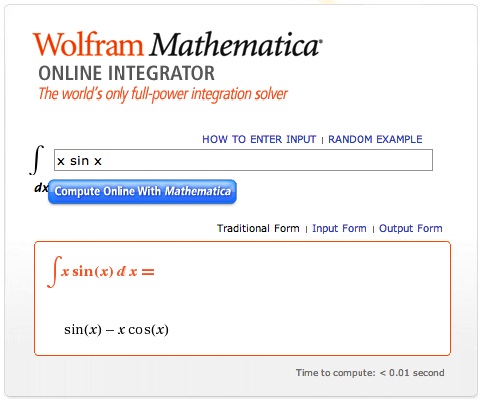
<math> ~4\pi \rho_c \biggl(\frac{R}{\pi}\biggr)^3 \int_0^\xi \xi\sin\xi ~d\xi </math> |
|
|
|
<math>~=</math> |
<math>~ \frac{4}{\pi^2} \rho_c R^3 [ \sin\xi - \xi\cos\xi ] \, . </math> |
Because <math>~\xi = \pi</math> at the surface of this spherical configuration — in which case the term inside the square brackets is <math>~\pi</math> — we conclude as well that the total mass of the configuration is,
<math> ~M = \frac{4}{\pi}\rho_c R^3 . </math>
Summary
From the above derivations, we can describe the properties of a spherical <math>~n</math> = 1 polytrope as follows:
- Mass:
- Given the density, <math>\rho_c</math>, and the radius, <math>R</math>, of the configuration, the total mass is,
<math>M = \frac{4}{\pi} \rho_c R^3 </math> ;
- and, expressed as a function of <math>M</math>, the mass that lies interior to radius <math>r</math> is,
<math>\frac{M_r}{M} = \frac{1}{\pi} \biggl[ \sin\biggl(\frac{\pi r}{R} \biggr) - \biggl(\frac{\pi r}{R} \biggr)\cos\biggl(\frac{\pi r}{R} \biggr) \biggr]</math> .
- Pressure:
- Given values for the pair of model parameters <math>( \rho_c , R )</math>, or <math>( M , R )</math>, or <math>( \rho_c , M )</math>, the central pressure of the configuration is,
<math>P_c = \frac{2 G}{\pi} \rho_c^2 R^2 = \frac{\pi G}{8}\biggl( \frac{M^2}{R^4} \biggr) = \biggl[ \frac{1}{2\pi} G^3 \rho_c^4 M^2 \biggr]^{1/3}</math> ;
- and, expressed in terms of the central pressure <math>P_c</math>, the variation with radius of the pressure is,
<math>P(r)= P_c \biggl[\frac{R}{\pi r} \sin\biggl(\frac{\pi r}{R}\biggr) \biggr]^2</math> .
- Enthalpy:
- Throughout the configuration, the enthalpy is given by the relation,
<math>H(r) = \frac{2 P(r)}{ \rho(r)} = \frac{GM}{R} \biggl[\frac{R}{\pi r} \sin\biggl(\frac{\pi r}{R}\biggr) \biggr]</math> .
- Gravitational potential:
- Throughout the configuration — that is, for all <math>r \leq R</math> — the gravitational potential is given by the relation,
<math>\Phi_\mathrm{surf} - \Phi(r) = H(r) = \frac{GM}{R} \biggl[\frac{R}{\pi r} \sin\biggl(\frac{\pi r}{R}\biggr) \biggr] </math> .
- Outside of this spherical configuration— that is, for all <math>r \geq R</math> — the potential should behave like a point mass potential, that is,
<math>\Phi(r) = - \frac{GM}{r} </math> .
- Matching these two expressions at the surface of the configuration, that is, setting <math>\Phi_\mathrm{surf} = - GM/R</math>, we have what is generally considered the properly normalized prescription for the gravitational potential inside a spherically symmetric, <math>~n</math> = 1 polytropic configuration:
<math>\Phi(r) = - \frac{G M}{R} \biggl\{ 1 + \biggl[\frac{R}{\pi r} \sin\biggl(\frac{\pi r}{R}\biggr) \biggr] \biggr\} </math> .
- Mass-Radius relationship:
- We see that, for a given value of <math>\rho_c</math>, the relationship between the configuration's total mass and radius is,
<math>M \propto R^3 ~~~~~\mathrm{or}~~~~~R \propto M^{1/3} </math> .
- Central- to Mean-Density Ratio:
- The ratio of the configuration's central density to its mean density is,
<math>\frac{\rho_c}{\bar{\rho}} = \biggl(\frac{\pi M}{4 R^3} \biggr)\biggl(\frac{3 M}{4 \pi R^3} \biggr) = \frac{\pi^2}{3} </math> .
| Figure 1: Mass vs. Radius for n = 1 polytrope |
|---|
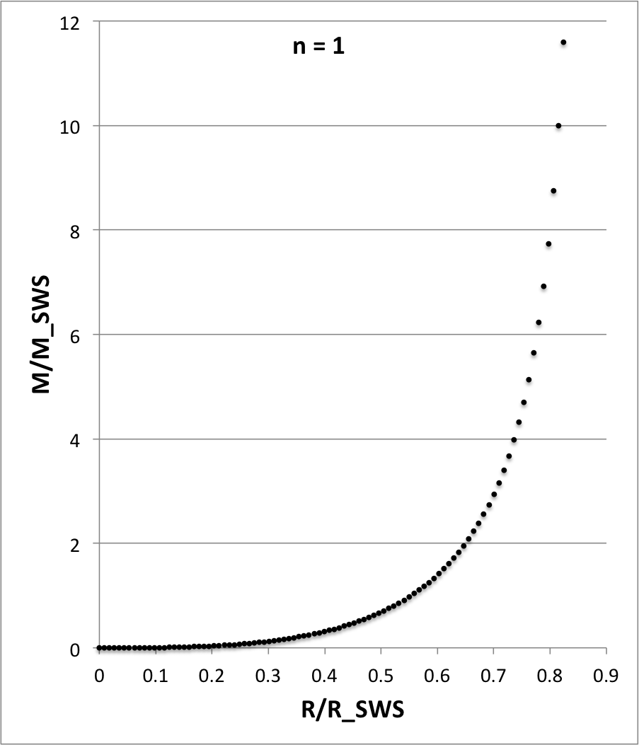 |
For the purposes of comparing the internal structure of configurations having different polytropic indexes — see, for example Figure 4, below — we have found it useful in each case to graphically illustrate how the normalized mass, <math>~M/M_\mathrm{SWS}</math>, varies with the normalized radius, <math>~R/R_\mathrm{SWS}</math>, where the definition of these two functions is drawn from an accompanying discussion of pressure-truncated polytropic configurations. In the case of an <math>~n=1</math> polytrope, both functions are expressible analytically; specifically, we have,
|
<math> ~\frac{R}{R_\mathrm{SWS}}\biggr|_{n=1} </math> |
<math>~\equiv~</math> |
<math> \biggl( \frac{1}{4\pi} \biggr)^{1/2} \xi \, ; </math> |
|
<math> ~\frac{M}{M_\mathrm{SWS}}\biggr|_{n=1} </math> |
<math>~=~</math> |
<math> \biggl( \frac{1}{4\pi} \biggr)^{1/2} \biggl[ \frac{\xi^2}{\theta_n} \biggl| \frac{d\theta_n}{d\xi} \biggr| ~\biggr]_{n=1} </math> |
|
|
<math>~=~</math> |
<math> \biggl( \frac{1}{4\pi} \biggr)^{1/2} \frac{\xi^3}{\sin\xi} \biggl[\frac{\sin\xi - \xi\cos\xi}{\xi^2} \biggr] </math> |
|
|
<math>~=~</math> |
<math> \biggl( \frac{1}{4\pi} \biggr)^{1/2} \xi \biggl[1 - \xi\cot\xi \biggr] \, . </math> |
As Figure 1 illustrates, this normalized mass increases monotonically with radius. Given that the surface of the configuration is associated with the parameter value, <math>~\xi = \pi</math>, we recognize that, at the surface, <math>~R/R_\mathrm{SWS} = \sqrt{\pi/4} \approx 0.8862269</math> and <math>~M/M_\mathrm{SWS}</math> formally climbs to infinity.
Published n = 1 Tabulations
| Published Tabulations of n = 1 Polytropic Structure (Primary E-Type Solution) | ||||||
|---|---|---|---|---|---|---|
|
Copied from p. 75 of Emden (1907) |
Copied from p. 73 of Horedt (2004) |
|||||
| <math>~\mathfrak{r}_1</math> | <math>~u_1</math> | <math>~- \frac{du_1}{d\mathfrak{r}_1}</math> | <math>~\xi</math> | <math>~\Theta_H</math> | <math>~- \frac{d\Theta_H}{d\xi}</math> | |
| <math>~0</math> | <math>~1</math> | <math>~0</math> | <math>~0</math> | <math>~1</math> | <math>~0</math> | |
| <math>~</math> | <math>~</math> | <math>~</math> | <math>~\tfrac{1}{10}</math> | <math>~9.983342\mathrm{E-01}</math> | <math>~3.330001\mathrm{E-02}</math> | |
| <math>~\tfrac{1}{4}</math> | <math>~0.98960</math> | <math>~0.08280</math> | <math>~</math> | <math>~</math> | <math>~</math> | |
| <math>~\tfrac{1}{2}</math> | <math>~0.95882</math> | <math>~0.16250</math> | <math>~\tfrac{1}{2}</math> | <math>~9.588511\mathrm{E-01}</math> | <math>~1.625370\mathrm{E-01}</math> | |
| <math>~\tfrac{3}{4}</math> | <math>~0.90886</math> | <math>~0.23623</math> | <math>~</math> | <math>~</math> | <math>~</math> | |
| <math>~1</math> | <math>~0.84148</math> | <math>~0.30117</math> | <math>~1</math> | <math>~8.414710\mathrm{E-01}</math> | <math>~3.011687\mathrm{E-01}</math> | |
| <math>~1 \tfrac{1}{4}</math> | <math>~0.75918</math> | <math>~0.35511</math> | <math>~</math> | <math>~</math> | <math>~</math> | |
| <math>~1\tfrac{1}{2}</math> | <math>~0.66500</math> | <math>~0.39622</math> | <math>~</math> | <math>~</math> | <math>~</math> | |
| <math>~2</math> | <math>~0.45464</math> | <math>~0.43541</math> | <math>2</math> | <math>~4.546487\mathrm{E-01}</math> | <math>~4.353978\mathrm{E-01}</math> | |
| <math>~2\tfrac{1}{2}</math> | <math>~0.23938</math> | <math>~0.41621</math> | <math>~</math> | <math>~</math> | <math>~</math> | |
| <math>~3</math> | <math>~0.04703</math> | <math>~0.34569</math> | <math>~3</math> | <math>~4.704000\mathrm{E-02}</math> | <math>~3.3456775\mathrm{E-01}</math> | |
| <math>~</math> | <math>~</math> | <math>~</math> | <math>~3.140</math> | <math>~5.072143\mathrm{E-04}</math> | <math>~3.186325\mathrm{E-01}</math> | |
| <math>~\pi</math> | <math>~0</math> | <math>~0.31831</math> | <math>~\pi</math> | <math>~0</math> | <math>~3.183099\mathrm{E-01}</math> | |
| <math>~3\tfrac{1}{4}</math> | <math>~-0.03330</math> | <math>~0.29564</math> | <math>~</math> | <math>~</math> | <math>~</math> | |
n = 5 Polytrope
Primary E-Type Solution
To derive the radial distribution of the Lane-Emden function <math>\Theta_H(r)</math> for an <math>~n</math> = 5 polytrope, we must solve,
<math>\frac{1}{\xi^2} \frac{d}{d\xi}\biggl( \xi^2 \frac{d\Theta_H}{d\xi} \biggr) = - (\Theta_H)^5</math> ,
subject to the above-specified boundary conditions. Following Emden (1907), [C67] (pp. 93-94) shows that by making the substitutions,
<math> \xi = \frac{1}{x} = e^{-t} \, ; ~~~~~\Theta_H = \biggl(\frac{x}{2}\biggr)^{1/2} z = \biggl(\frac{1}{2}e^t\biggr)^{1/2}z \, , </math>
the differential equation can be rewritten as,
<math> \frac{d^2 z}{dt^2} = \frac{1}{4}z (1 - z^4) \, . </math>
This equation has the solution,
<math> z = \pm \biggl[ \frac{12 C e^{-2t}}{(1 + C e^{-2t})^2} \biggr]^{1/4} \, , </math>
that is,
<math> \Theta_H = \biggl[ \frac{3 C }{(1 + C \xi^2)^2} \biggr]^{1/4} \, . </math>
where <math>C</math> is an integration constant. Because <math>\Theta_H</math> must go to unity when <math>\xi = 0</math>, we see that <math>C=1/3</math>. Hence,
<math> \Theta_H = \biggl[ 1 + \frac{1}{3}\xi^2 \biggr]^{-1/2} \, . </math>
From this Lane-Emden function solution, we obtain,
<math> \frac{\rho}{\rho_c} = \Theta_H^5 = \biggl[ 1 + \frac{1}{3}\xi^2 \biggr]^{-5/2} \, , </math>
and,
<math> \frac{P}{P_c} = \biggr(\frac{\rho}{\rho_c}\biggr)^{6/5} = \biggl[ 1 + \frac{1}{3}\xi^2 \biggr]^{-3} \, . </math>
Notice that, for this polytropic structure, the density and pressure don't go to zero until <math>\xi \rightarrow \infty</math>. Hence, <math>\xi_1 = \infty</math>. However, the radial scale length,
<math> a_5 = \biggr[ \frac{1}{4\pi G} \biggl( \frac{H_c}{\rho_c} \biggr) \biggr]^{1/2} = \biggr[ \frac{(n+1)K}{4\pi G} \rho_c^{(1/n - 1)} \biggr]^{1/2} = \biggr[ \frac{3K}{2\pi G} \biggr]^{1/2} \rho_c^{-2/5} \, . </math>
Hence,
|
<math> M_r(\xi) </math> |
<math>=</math> |
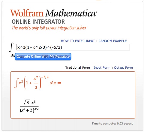
<math> 4\pi \rho_c a_5^3 \int_0^\xi \xi^2 \biggl[ 1 + \frac{1}{3}\xi^2 \biggr]^{-5/2} d\xi </math> | |
|
|
<math>=</math> |
<math> 4\pi \biggr[ \frac{3K}{2\pi G} \biggr]^{3/2} \rho_c^{-1/5} ~\biggl\{ \frac{\sqrt{3} \xi^3}{(3 + \xi^2)^{3/2}} \biggr\} </math> |
|
|
|
<math>=</math> |
<math> \biggr[ \frac{2\cdot 3^4 K^3}{\pi G^3} \biggr]^{1/2} \rho_c^{-1/5} ~\{ \xi^3 ( 3 + \xi^2 )^{-3/2} \} \, . </math> |
The function of <math>\xi</math> inside the curly brackets of this last expression goes to unity as <math>\xi \rightarrow \infty</math>, so the integrated mass is finite even though the configuration extends to infinity. Specifically, the total mass is,
<math>M = \biggr[ \frac{2\cdot 3^4 K^3}{\pi G^3} \biggr]^{1/2} \rho_c^{-1/5} \, .</math>
We can invert this formula to obtain an expression for <math>K</math> in terms of <math>M</math> and <math>\rho_c</math>, namely,
<math> K = \biggr[ \frac{\pi M^2 G^3}{2\cdot 3^4} \biggr]^{1/3} \rho_c^{2/15} \, . </math>
This, in turn, means that the central pressure,
<math> P_c = K\rho_c^{6/5} = \biggr[ \frac{\pi M^2 G^3}{2\cdot 3^4} \biggr]^{1/3} \rho_c^{4/3} \, , </math>
and,
<math> H_c = \frac{6P_c}{\rho_c} = \biggr[ \frac{2^2 \pi M^2 G^3}{3} \biggr]^{1/3} \rho_c^{1/3} \, . </math>
| Figure 2: Mass vs. Radius for n = 5 polytrope |
|---|
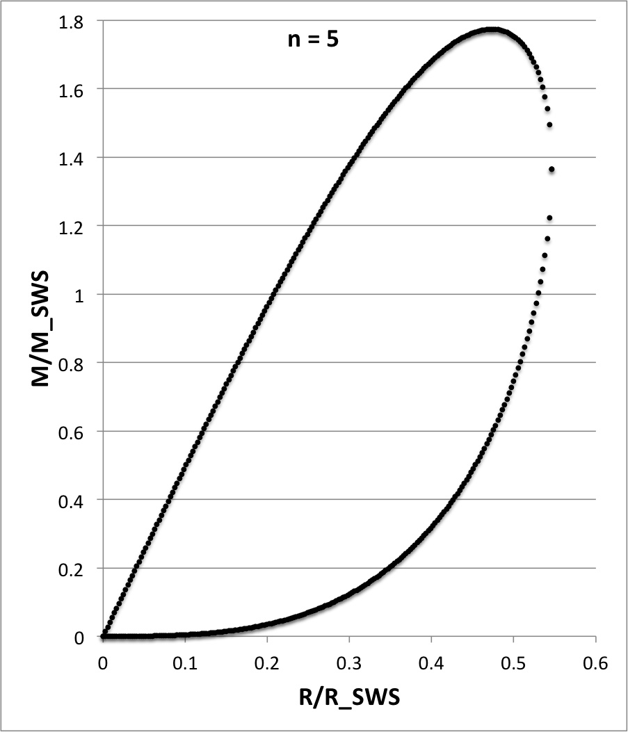 |
For the purposes of comparing the internal structure of configurations having different polytropic indexes — see, for example Figure 4, below — we have found it useful in each case to graphically illustrate how the normalized mass, <math>~M/M_\mathrm{SWS}</math>, varies with the normalized radius, <math>~R/R_\mathrm{SWS}</math>, where the definition of these two functions is drawn from an accompanying discussion of pressure-truncated polytropic configurations. In the case of an <math>~n=5</math> polytrope, both functions are expressible analytically; specifically, we have,
|
<math> ~\frac{R}{R_\mathrm{SWS}} </math> |
<math>~=~</math> |
<math> \biggl( \frac{5}{4\pi} \biggr)^{1/2} \biggl[ \xi \theta^{2} \biggr]_{n=5} </math> |
|
|
<math>~=~</math> |
<math> \biggl( \frac{5}{4\pi} \biggr)^{1/2} \xi \biggl[1 + \frac{\xi^2}{3} \biggr]^{-1} </math> |
|
|
<math>~=~</math> |
<math> \biggl( \frac{5}{4\pi} \biggr)^{1/2} \biggl[\frac{3\xi}{3 + \xi^2} \biggr] \, ; </math> |
|
<math> ~\frac{M}{M_\mathrm{SWS}} </math> |
<math>~\equiv~</math> |
<math>~ \biggl( \frac{5^3}{4\pi} \biggr)^{1/2} \biggl[\theta \xi^2 \biggl| \frac{d\theta}{d\xi} \biggr| ~\biggr]_{n=5} </math> |
|
|
<math>~\equiv~</math> |
<math>~ \biggl( \frac{5^3}{4\pi} \biggr)^{1/2} \biggl\{\xi^2 \biggl[1 + \frac{\xi^2}{3}\biggr]^{-1 / 2} \frac{\xi}{3} \biggl[1 + \frac{\xi^2}{3}\biggr]^{-3 / 2} \biggr\} </math> |
|
|
<math>~\equiv~</math> |
<math>~ \biggl( \frac{5^3}{4\pi} \biggr)^{1/2} \frac{3\xi^3}{(3 + \xi^2)^2}\, . </math> |
As Stahler has pointed out, for an <math>~n = 5</math> polytrope, this mass-radius relation can also be precisely couched in the form of a quadratic equation, namely,
|
<math>~0</math> |
<math>~=</math> |
<math>~ \biggl( \frac{M}{M_\mathrm{SWS}} \biggr)^2 - 5 \biggl( \frac{M}{M_\mathrm{SWS}} \biggr)\biggl( \frac{R}{R_\mathrm{SWS}} \biggr) + \frac{2^2 \cdot 5 \pi}{3} \biggl( \frac{R}{R_\mathrm{SWS}} \biggr)^4 </math> |
|
<math>~\Rightarrow ~~~ \frac{M}{M_\mathrm{SWS}}</math> |
<math>~=</math> |
<math>~ \frac{5}{2} \biggl( \frac{R}{R_\mathrm{SWS}} \biggr) \biggl[ 1 \pm \sqrt{1- \frac{2^4 \pi}{3\cdot 5}\biggl( \frac{R}{R_\mathrm{SWS}} \biggr)^2} \biggr] \, . </math> |
As Figure 2 illustrates, this mass-radius relationship exhibits two turning points: The maximum radius occurs at coordinate location,
<math>~\biggl[ \frac{R}{R_\mathrm{SWS}}, \frac{M}{M_\mathrm{SWS}}\biggr]_\mathrm{R\_turn} = \biggl[ \biggl( \frac{3\cdot 5}{2^4 \pi} \biggr)^{1 / 2}, \biggl( \frac{3\cdot 5^3}{2^6 \pi} \biggr)^{1 / 2} \biggr] \approx \biggl[ 0.5462742, 1.3656855\biggr] \, ;</math>
and the maximum mass occurs at coordinate location,
<math>~\biggl[ \frac{R}{R_\mathrm{SWS}}, \frac{M}{M_\mathrm{SWS}}\biggr]_\mathrm{M\_turn} = \biggl[ \biggl( \frac{3^2\cdot 5}{2^6 \pi} \biggr)^{1 / 2}, \biggl( \frac{3^4\cdot 5^3}{2^{10} \pi} \biggr)^{1 / 2} \biggr] \approx \biggl[ 0.4730873, 1.7740776\biggr] \, .</math>
Published n = 5 Tabulations
| Published Tabulations of n = 5 Polytropic Structure (Primary E-Type Solution) | ||||||
|---|---|---|---|---|---|---|
|
Copied from p. 76 of Emden (1907) |
Copied from p. 75 of Horedt (2004) |
|||||
| <math>~\mathfrak{r}_1</math> | <math>~u_1</math> | <math>~- \frac{du_1}{d\mathfrak{r}_1}</math> | <math>~\xi</math> | <math>~\Theta_H</math> | <math>~- \frac{d\Theta_H}{d\xi}</math> | |
| <math>~0</math> | <math>~1</math> | <math>~0</math> | <math>~0</math> | <math>~1</math> | <math>~0</math> | |
| <math>~</math> | <math>~</math> | <math>~</math> | <math>~\tfrac{1}{10}</math> | <math>~9.983375\mathrm{E-01}</math> | <math>~3.316736\mathrm{E-02}</math> | |
| <math>~\tfrac{1}{4}</math> | <math>~0.98974</math> | <math>~0.08079</math> | <math>~</math> | <math>~</math> | <math>~</math> | |
| <math>~\tfrac{2}{4}</math> | <math>~0.96078</math> | <math>~0.14781</math> | <math>~\tfrac{1}{2}</math> | <math>~9.607689\mathrm{E-01}</math> | <math>~1.478106\mathrm{E-01}</math> | |
| <math>~\tfrac{3}{4}</math> | <math>~0.91768</math> | <math>~0.19320</math> | <math>~</math> | <math>~</math> | <math>~</math> | |
| <math>~1</math> | <math>~0.86602</math> | <math>~0.21650</math> | <math>~1</math> | <math>~8.660254\mathrm{E-01}</math> | <math>~2.165064\mathrm{E-01}</math> | |
| <math>~\tfrac{3}{2}</math> | <math>~0.75593</math> | <math>~0.21598</math> | <math>~</math> | <math>~</math> | <math>~</math> | |
| <math>~2</math> | <math>~0.65465</math> | <math>~0.18704</math> | <math>~</math> | <math>~</math> | <math>~</math> | |
| <math>~\tfrac{5}{2}</math> | <math>~0.56950</math> | <math>~0.15392</math> | <math>~</math> | <math>~</math> | <math>~</math> | |
| <math>~3</math> | <math>~0.50000</math> | <math>~0.12500</math> | <math>~</math> | <math>~</math> | <math>~</math> | |
| <math>~\tfrac{7}{2}</math> | <math>~0.44353</math> | <math>~0.10180</math> | <math>~</math> | <math>~</math> | <math>~</math> | |
| <math>~4</math> | <math>~0.39736</math> | <math>~0.08365</math> | <math>~</math> | <math>~</math> | <math>~</math> | |
| <math>~5</math> | <math>~0.32733</math> | <math>~0.05845</math> | <math>~5</math> | <math>~3.273268\mathrm{E-01}</math> | <math>~5.845122\mathrm{E-02}</math> | |
| <math>~6</math> | <math>~0.27735</math> | <math>~0.04267</math> | <math>~</math> | <math>~</math> | <math>~</math> | |
| <math>~7</math> | <math>~0.24020</math> | <math>~0.03233</math> | <math>~</math> | <math>~</math> | <math>~</math> | |
| <math>~8</math> | <math>~0.21160</math> | <math>~0.02527</math> | <math>~</math> | <math>~</math> | <math>~</math> | |
| <math>~10</math> | <math>~0.17066</math> | <math>~0.01657</math> | <math>~10</math> | <math>~1.706640\mathrm{E-01}</math> | <math>~1.656932\mathrm{E-02}</math> | |
| <math>~12</math> | <math>~0.14286</math> | <math>~0.01166</math> | <math>~</math> | <math>~</math> | <math>~</math> | |
| <math>~16</math> | <math>~0.10763</math> | <math>~0.00665</math> | <math>~</math> | <math>~</math> | <math>~</math> | |
| <math>~20</math> | <math>~0.08628</math> | <math>~0.00428</math> | <math>~</math> | <math>~</math> | <math>~</math> | |
| <math>~30</math> | <math>~0.05764</math> | <math>~0.00192</math> | <math>~</math> | <math>~</math> | <math>~</math> | |
| <math>~</math> | <math>~</math> | <math>~</math> | <math>~50</math> | <math>~3.462025\mathrm{E-02}</math> | <math>~6.915751\mathrm{E-04}</math> | |
| <math>~</math> | <math>~</math> | <math>~</math> | <math>~100</math> | <math>~1.731791\mathrm{E-02}</math> | <math>~1.731272\mathrm{E-04}</math> | |
| <math>~</math> | <math>~</math> | <math>~</math> | <math>~500</math> | <math>~3.464081\mathrm{E-03}</math> | <math>~6.928079\mathrm{E-06}</math> | |
| <math>~</math> | <math>~</math> | <math>~</math> | <math>~1000</math> | <math>~1.732048\mathrm{E-03}</math> | <math>~1.732043\mathrm{E-06}</math> | |
| <math>~</math> | <math>~</math> | <math>~</math> | <math>~\infty</math> | <math>~0.000000\mathrm{E+00}</math> | <math>~0.000000\mathrm{E+00}</math> | |
Srivastava's F-Type Solution
Demonstration of Function's Validity
In a short paper, S. Srivastava (1968, ApJ, 136, 680) presents another, analytically prescribable solution to the Lane-Emden equation of index <math>~n = 5</math> that we will call upon in our discussion of one category of bipolytropic configurations. Rather than repeat Srivastava's derivation here, we will simply specify his functional solution then demonstrate that it satisfies the Lane-Emden equation. Srivastiva's Lane-Emden function is (see his equations 12 & 13),
|
<math>~\theta_{5F}</math> |
<math>~=</math> |
<math>~\frac{\sin[\ln(A\xi)^{1/2})]}{\xi^{1/2}\{3-2\sin^2[\ln(A\xi)^{1/2}]\}^{1/2}} \, ,</math> |
where, <math>~A</math> is an arbitrary (positive) constant. Adopting the shorthand notation,
<math>\Delta \equiv \ln(A\xi)^{1/2}\, ,</math>
and, recognizing that,
|
<math>\frac{d}{d\ln(A\xi)}\biggl[ \ln(A\xi)^{1/2} \biggr] = \frac{1}{2}</math> |
<math>~\Rightarrow~</math> |
<math>~\frac{d\Delta}{d\xi} = \frac{1}{2\xi} \, , </math> |
the first derivative of Srivastava's Lane-Emden function is,
|
<math>~\frac{d\theta_{5F}}{d\xi}</math> |
<math>~=</math> |
<math>~ \frac{\cos\Delta}{2\xi^{3/2}(3-2\sin^2\Delta)^{1/2}} - \frac{\sin\Delta}{2\xi^{3/2}(3-2\sin^2\Delta)^{1/2}} + \frac{\sin^2\Delta \cos\Delta }{\xi^{3/2}(3-2\sin^2\Delta)^{3/2}} </math> |
|
|
<math>~=</math> |
<math>~ \frac{1}{2\xi^{3/2}(3-2\sin^2\Delta)^{3/2}} \biggl[ (\cos\Delta - \sin\Delta ) (3-2\sin^2\Delta) + 2\sin^2\Delta\cos\Delta \biggr] </math> |
|
|
<math>~=</math> |
<math>~ \frac{3\cos\Delta-3\sin\Delta + 2\sin^3\Delta }{2\xi^{3/2}(3-2\sin^2\Delta)^{3/2}} \, . </math> |
Hence, the left-hand-side of the,
Lane-Emden Equation
|
<math>~\frac{1}{\xi^2} \frac{d}{d\xi}\biggl( \xi^2 \frac{d\Theta_H}{d\xi} \biggr) = - \Theta_H^n</math> |
is,
|
LHS |
<math>~=</math> |
<math>~ \frac{1}{\xi^2}\frac{d}{d\xi}\biggl[ \frac{\xi^{1/2}(3\cos\Delta-3\sin\Delta + 2\sin^3\Delta )}{2(3-2\sin^2\Delta)^{3/2}} \biggr] </math> |
|
|
<math>~=</math> |
<math>~ \frac{1}{\xi^2}\biggl[ \frac{(3\cos\Delta-3\sin\Delta + 2\sin^3\Delta )}{4\xi^{1/2}(3-2\sin^2\Delta)^{3/2}} + \frac{(-3\sin\Delta-3\cos\Delta + 6\sin^2\Delta \cos\Delta )}{4\xi^{1/2}(3-2\sin^2\Delta)^{3/2}} </math> |
|
|
|
<math>~ + \frac{3(3\cos\Delta-3\sin\Delta + 2\sin^3\Delta )\sin\Delta \cos\Delta}{2\xi^{1/2}(3-2\sin^2\Delta)^{5/2}} \biggr] </math> |
|
|
<math>~=</math> |
<math>~2^{-2}\xi^{-5/2}(3-2\sin^2\Delta)^{-5/2} [ (3-2\sin^2\Delta) (3\cos\Delta-3\sin\Delta + 2\sin^3\Delta ) </math> |
|
|
|
<math>~+ (3-2\sin^2\Delta) (-3\sin\Delta-3\cos\Delta + 6\sin^2\Delta \cos\Delta ) + 6(3\cos\Delta-3\sin\Delta + 2\sin^3\Delta )\sin\Delta \cos\Delta ]</math> |
|
|
<math>~=</math> |
<math>~2^{-2}\xi^{-5/2}(3-2\sin^2\Delta)^{-5/2} [ (3-2\sin^2\Delta) (-6\sin\Delta + 2\sin^3\Delta + 6\sin^2\cos\Delta) </math> |
|
|
|
<math>~ + 6(3\cos\Delta-3\sin\Delta + 2\sin^3\Delta )\sin\Delta \cos\Delta ]</math> |
|
|
<math>~=</math> |
<math>~2^{-2}\xi^{-5/2}(3-2\sin^2\Delta)^{-5/2} [ -18\sin\Delta + 6\sin^3\Delta + 18\sin^2\cos\Delta + 12\sin^3\Delta - 4\sin^5\Delta -12\sin^4\cos\Delta </math> |
|
|
|
<math>~ + 18\sin\Delta \cos^2\Delta-18\sin^2\Delta \cos\Delta + 12\sin^4\Delta \cos\Delta ]</math> |
|
|
<math>~=</math> |
<math>~2^{-2}\xi^{-5/2}(3-2\sin^2\Delta)^{-5/2}[ -4\sin^5\Delta ] </math> |
|
|
<math>~=</math> |
<math>~- \theta_{5F}^5 \, . </math> |
This demonstrates that Srivastava's function satisfies the Lane-Emden equation of index <math>~n=5</math>.
Function Properties
The function, <math>~\theta_{5F}</math>, looks like a damped oscillator with the following specific properties:
- As <math>~\xi</math> increases from zero, the function oscillates with an ever increasing period; the function goes through zero when <math>~\Delta = \pm \pi m</math> (m is an integer), that is, when <math>~(A\xi) = e^{\pm 2\pi m}</math>.
- The amplitude of the oscillation drops approximately as <math>~\xi^{-1/2}</math>.
- In an astrophysical context, the function can be used as a physically realistic representation of a spherical shell inside of a self-gravitating configuration only over the interval of a single oscillation for which <math>~\theta_{5F}</math> is positive (ensuring that the mass density is everywhere positive) and, at the same time, <math>~d\theta_{5F}/d\xi</math> is negative (ensuring that the density and pressure are a decreasing function of the radial coordinate). In the following example, the astrophysically relevant segment of the function is identified with the parameter interval, <math>~\xi_\mathrm{crit} \le (A\xi) \le e^{2\pi}</math>.
Example Interval
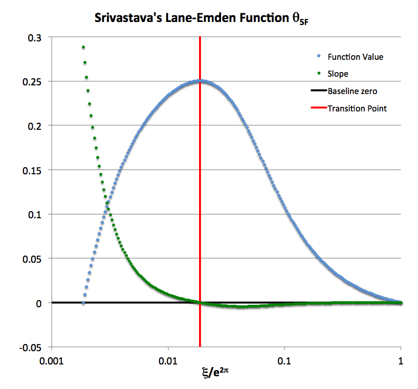
As an example, let's set <math>~A=1</math> and examine the oscillation interval between <math>~m=0</math> and <math>~m=1</math>, that is, over the range, <math>~0 \le \Delta \le \pi</math> which corresponds to the parameter interval <math>~\xi = [1, e^{2\pi}]</math>. The denominator of <math>~\theta_{5F}</math> is positive for all values of <math>~\xi</math> and, over this specified interval, the numerator of <math>~\theta_{5F}</math> is also always positive. The blue curve in the following figure presents a plot of <math>~\theta_{5F}(x)</math> and the green curve presents a plot of the first derivative (the slope) of the function <math>~d\theta_{5F}(x)/d\xi</math> over the desired interval, where <math>~x \equiv \xi/e^{2\pi}</math>; note that the horizontal axis is shown in logarithmic units.
| Figure 3: Segment of <math>~\theta_{5F}</math> Function as derived by S. Srivastava (1968, ApJ, 136, 680) |
|---|
At both ends of the chosen parameter interval — that is, at <math>~\Delta = 0</math> and at <math>~\Delta = \pi</math> — the function <math>~\theta_{5F} = 0</math> and, correspondingly as depicted in the figure, the blue curve touches the horizontal axis. At the beginning of the interval (<math>~\Delta =0</math>), the slope of the function and, correspondingly, the green curve, has the (positive) value,
|
<math>~\frac{d\theta_{5F}}{d\xi}</math> |
<math>~=</math> |
<math>~ \frac{3\cos(0)-3\sin(0) + 2\sin^3(0) }{2\xi^{3/2}[3-2\sin^2(0)]^{3/2}} = \frac{3}{2(3^{3/2})} = (2^2 \cdot 3)^{-1/2} \approx 0.28868 \, . </math> |
At the end of the interval (<math>~\Delta=\pi</math>), the slope of the function as well as the green curve, has the (negative) value,
|
<math>~\frac{d\theta_{5F}}{d\xi}</math> |
<math>~=</math> |
<math>~ \frac{3\cos(\pi)-3\sin(\pi) + 2\sin^3(\pi) }{2\xi^{3/2}[3-2\sin^2(\pi)]^{3/2}} = \frac{-3}{2e^{3\pi}(3^{3/2})} = -e^{-3\pi} (2^2 \cdot 3)^{-1/2} \approx -2.3296 \times 10^{-5} \, . </math> |
Over this interval, <math>~\theta_{5F}</math> reaches its maximum when the slope of the function is zero, that is, at the value of <math>~\Delta</math> where,
|
<math>~ 0 </math> |
<math>~=</math> |
<math>~3\cos\Delta -3\sin\Delta +2(1-\cos^2\Delta)\sin\Delta</math> |
|
|
<math>~=</math> |
<math>~3\cos\Delta -\sin\Delta -2\cos^2\Delta \sin\Delta</math> |
|
<math>~\Rightarrow ~~~~1</math> |
<math>~=</math> |
<math>~3\cot\Delta -2\cos^2\Delta \, .</math> |
Rewriting both of these trigonometric functions in terms of the tangent function and adopting the shorthand notation,
<math>~y \equiv \tan\Delta \, ,</math>
this condition becomes,
|
<math>~1</math> |
<math>~=</math> |
<math>~\frac{3}{y} -\frac{2}{1+y^2} </math> |
|
<math>~\Rightarrow ~~~~ y(y^2 + 1)</math> |
<math>~=</math> |
<math>~3(y^2+1) - 2y </math> |
|
<math>~\Rightarrow ~~~~ y^3 - 3y^2 + 3y - 3</math> |
<math>~=</math> |
<math>~0 \, .</math> |
|
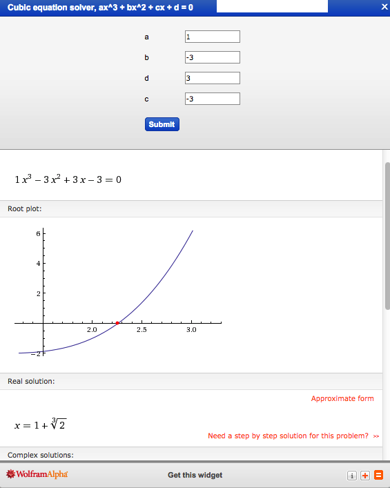
ASIDE: As is well known and documented — see, for example Wolfram MathWorld or Wikipedia's discussion of the topic — the roots of any cubic equation can be determined analytically. In order to evaluate the root(s) of our particular cubic equation, we have drawn from the utilitarian online summary provided by Eric Schechter at Vanderbilt University. For a cubic equation of the general form, <math>~ay^3 + by^2 + cy + d = 0 \, ,</math> a real root is given by the expression, <math>~ y = p + \{q + [q^2 + (r-p^2)^3]^{1/2}\}^{1/3} + \{q - [q^2 + (r-p^2)^3]^{1/2}\}^{1/3} \, ,</math> where, <math>~p \equiv -\frac{b}{3a} \, ,</math> <math>~q \equiv \biggl[p^3 + \frac{bc-3ad}{6a^2} \biggr] \, ,</math> and <math>~r=\frac{c}{3a} \, .</math> In our particular case, <math>~a =1\, ,</math> <math>~b =-3\, ,</math> <math>~c = +3 \, ,</math> and <math>~d = - 3 \, .</math> <math>~p = q = r = + 1 \, ,</math> which implies that the real root is,
(There is also a pair of imaginary roots, but they are irrelevant in the context of our overarching astrophysical discussion.) Just for fun, we have also used WolframAlpha's online "cubic equation solver" widget to find the root(s) of our specific cubic equation. Clicking on the thumbnail image provided here, on the right, displays the key result that was returned by this WolframAlpha widget. |
The single, real root of this cubic equation is,
<math>~y = 1 + 2^{1/3} \, ,</math>
which corresponds to,
<math>~\Delta = \tan^{-1}(1 + 2^{1/3}) \, .</math>
Hence, over this example interval, the maximum of Srivastava's <math>~\theta_{5F}</math> function — and, hence also, the location at which the function's slope transitions from positive to negative values (denoted by the vertical red line in the above figure) — occurs at,
<math>\xi_\mathrm{crit} \equiv e^{2\tan^{-1}(1+2^{1/3})} = 10.05836783\, .</math>
The corresponding value of the function at this critical radial location is,
<math>\theta_{5F}|_\mathrm{max} \equiv \theta_{5F}(\xi_\mathrm{crit}) = (1+2^{1/3})[3 + (1+2^{1/3})^2]^{-1/2} e^{-\tan^{-1}(1+2^{1/3})} = 0.250260848 \, .</math>
This agrees precisely with the determination made by J. O. Murphy (1983) — see the excerpts from his paper displayed in the following boxed-in image — that the portion of the <math>~\theta_{5F}</math> function that falls in the interval <math>~1 \le (A\xi) < \xi_\mathrm{crit}</math> (the segment of the blue curve that lies to the left of the vertical red line in the above figure) is unphysical because the slope of the function is positive throughout that interval.
|
Equation and text extracted† from p. 177 of J. O. Murphy (1983)
"Composite and Analytical Solutions of the Lane-Emden Equation with Polytropic Indices N = 1 and N = 5"
Proc. Astronomical Soc. Australia, vol. 5, pp. 175-179 © Astronomical Society of Australia | |
|
|
| †Equations and text displayed here, with presentation order & layout modified from the original publication. |
On the other hand, the segment that falls in the interval, <math>~\xi_\mathrm{crit} \le (A\xi) \le e^{2\pi}</math>, whose function values lie in the range, <math>~\theta_{5F}|_\mathrm{max} \ge (A^{-1/2} \theta_{5F}) \ge 0</math> — that is, the segment of the blue curve that lies to the right of the vertical red line in the above figure — can be used to describe the <math>~n=5</math> "envelope" of a bipolytropic configuration because the function value is positive while it's first derivative is negative.
Other (All) Solutions
In a very clearly written article titled, All Solutions of the n = 5 Lane-Emden Equation, Patryk Mach (2012, J. Math. Phys., 53, 062503) has pointed out that there are other families of solutions to the Lane-Emden equation of index, <math>~n=5</math>, in addition to the two solutions that have just been detailed, which he includes as his equations (3) and (5):
|
Equations extracted† from pp. 062503-1 & -2 of Mach (2012)
"All Solutions of the n = 5 Lane-Emden Equation"
Journal of Mathematical Physics, vol. 53, pp. 062503-062503-6 © American Institute of Physics | ||||||||
|
||||||||
| †Equations displayed here, with layout modified from the original publication. |
For completeness, Mach mentions a well-known solution that works for all indexes, <math>~n > 3</math>, which we have discussed separately in the context of power-law density distributions, namely,
<math>\theta^n(\xi) = \frac{\rho}{\rho_c} = \biggl[ \frac{2(n-3)}{(n-1)^2} \biggr]^{n/(n-1)} \xi^{- 2n/(n-1)} \, . </math>
In addition, Mach identifies the rarely referenced work of H. Goenner & P. Havas (2000, J. Math. Phys., 41, 7029), which presents a family of solutions that is expressed in terms of the Weierstrass elliptic function; and he derives a new family of solutions — see equation (10) in his §2.1 — that can be expressed entirely in terms of Jacobi elliptic functions. Mach's new solutions, in particular, are oscillatory (like Srivastava's solution) but have no zeros, so in isolation they are not likely to be useful for astrophysical models. But, as Mach suggests, they "can be used in composite stellar models on the same footing as Srivastava's solution" — see our accompanying description of a composite model using Srivastava's solution.
Numerical Solutions
Here we explain how an Excel workbook can be used to numerically solve the Lane-Emden equation, evaluating the Lane-Emden function across a one-dimensional, discrete grid.
Techniques
HSCF Technique
On the first spreadsheet within the workbook, we establish the following columns of number:
- Column A: Labeled <math>~r_i/R</math> (for i between 1 and N), that represents a discrete radial grid of spacing, <math>~~\Delta = (N-1)^{-1}</math>; each row gives the radial coordinate location of the ith zone, starting from <math>~r_1/R = 0</math> and ending at <math>~r_N/R = 1</math>.
- Column B: Labeled <math>~\mathrm{rhf}_i</math> (for i between 1 and N-1); each row gives the radial coordinate of the mid-point of a grid zone.
- Column C: Labeled <math>~\rho_i</math> (for i between 1 and N-1); each row provides an initial guess for the mass-density of the grid zone. Usually it is sufficient to guess, <math>~\rho_i = 1</math> throughout. For an <math>~n=0</math> polytrope, this proves also to be the correct final density profile.
- Column D: Labeled <math>~M_i</math> (for i between 1 and N); the ith row gives the integrated mass enclosed interior to the radial grid coordinate, <math>~r_i/R</math>. Specifically, <math>~M_1 = 0</math>, and thereafter, beginning with zone, <math>~i = 2</math>,
- Note that, <math>~M_\mathrm{tot} = M_N \, .</math>
- Column E: Labeled <math>~g_i</math> (for i between 2 and N); each row tabulates the inwardly directed gravitational acceleration that is felt at the outer edge of each grid zone. Specifically,
- Column F: Labeled <math>~\Phi_i</math> (for i between 1 and N); each row gives the value of the gravitational potential at the mid-point of a grid zone. Here, we start by specifying the value of the potential just (specifically, half a radial grid-zone) outside the surface of the configuration, where it should be, <math>~\Phi_N = -GM_\mathrm{tot}/(1+\Delta/2)</math>. Then, working from the surface, inward and, given that, <math>~g = d\Phi/dr</math>, we use the corresponding finite-difference representation of the radial derivative and set,
- Note that the value of the gravitational potential at the surface is not <math>~\Phi_N</math> but, rather, must be <math>~\Phi_\mathrm{surf} = -GM_\mathrm{tot}/R</math>.
- Furthermore, note that a lop-sided Taylor-series expansion about the center of the configuration provides the following good approximation to the gravitational potential at the center: <math>~\Phi_c \approx (9\Phi_1 - \Phi_2)/8</math>.
- Note as well that all of these numerically determined values of the gravitational potential can be checked against the known analytic expression for the radial profile of the potential in a uniform-density sphere.
- Column G: Labeled <math>~H_i</math> (for i between 1 and N-1); each row provides the value of the fluid enthalpy at the center of a grid cell. Adopting the convention that the enthalpy is zero at the surface of the configuration, and given that the enthalpy and the gravitational potential must sum to zero throughout the configuration, we have,
- At the center of the configuration, we have, <math>~H_c = \Phi_\mathrm{surf} - \Phi_c</math>.
- Column H: Labeled <math>~H_\mathrm{norm}</math> (for i between 1 and N-1); each row provides the value of the fluid enthalpy, renormalized to the central value, specifically,
<math>~\mathrm{rhf}_i \equiv \frac{1}{2}\biggr[\frac{r_i}{R} + \frac{r_{i+1}}{R} \biggr] \, .</math>
<math>~M_i = M_{i-1} + \frac{4\pi \rho_{i-1}}{3}\biggl[ \biggl(\frac{r_{i}}{R} \biggr)^3 - \biggl(\frac{r_{i-1}}{R} \biggr)^3 \biggr] \, .</math>
<math>g_i = \frac{GM_i}{ (r_i/R)^2} \, .</math>
|
<math>~\frac{\Phi_i - \Phi_{i-1}}{\Delta} </math> |
<math>~=</math> |
<math>~g_i </math> |
|
<math>~\Rightarrow ~~~ \Phi_{i-1} </math> |
<math>~=</math> |
<math>~ \Phi_i - g_i \Delta \, .</math> |
<math>H_i = \Phi_\mathrm{surf} - \Phi_i \, .</math>
<math>~[H_\mathrm{norm}]_i = \frac{H_i}{H_c} \, .</math>
The second spreadsheet within the workbook should be initially created by generating a copy of the first spreadsheet. Then:
- Column C: Labeled <math>~\rho_i</math> (for i between 1 and N-1); generate a new, improved guess for the normalized mass-density at each grid zone based on the corresponding value of the normalized enthalpy from the previous spreadsheet/iteration. Specifically, given that the relationship between the density and enthalpy in a polytrope of index, <math>~n</math>, is, <math>~\rho \propto H^n</math>, we should set,
<math>~\biggl\{ \frac{\rho_i}{\rho_c} \biggr\}_\mathrm{sheet2}= \biggr\{[H_\mathrm{norm}]_i^n \biggr\}_\mathrm{sheet1} \, .</math>
Straight Numerical Integration
The above governing relation may be rewritten as,
|
<math>~ \xi \theta^{} + 2 \theta^' </math> |
<math>~=</math> |
<math>~- \xi \theta^n \, .</math> |
We'll adopt the following finite-difference approximations for the first and second derivatives on a grid of radial spacing, <math>~\Delta_\xi</math>:
|
<math>~\theta_i'</math> |
<math>~\approx</math> |
<math>~\frac{\theta_+ - \theta_-}{2\Delta_\xi}</math> |
and,
|
<math>~\theta_i</math> |
<math>~\approx</math> |
<math>~\frac{\theta_+ - 2\theta_i +\theta_-}{\Delta_\xi^2} \, .</math> |
Our finite-difference approximation of the governing equation is, then,
|
<math>~\xi_i \biggl[ \frac{\theta_+ - 2\theta_i +\theta_-}{\Delta_\xi^2} \biggr] + 2\biggl[ \frac{\theta_+ - \theta_-}{2\Delta_\xi}\biggr] </math> |
<math>~=</math> |
<math>~- \xi_i \theta_i^n </math> |
|
<math>~\Rightarrow ~~~ \xi_i [ \theta_+ - 2\theta_i +\theta_-] + \Delta_\xi [ \theta_+ - \theta_- ] </math> |
<math>~=</math> |
<math>~- \Delta_\xi^2\xi_i \theta_i^n </math> |
|
<math>~\Rightarrow ~~~ \theta_+ </math> |
<math>~=</math> |
<math>~\frac{2\xi_i \theta_i + \theta_-(\Delta_\xi - \xi_i) - \Delta_\xi^2\xi_i \theta_i^n }{\Delta_\xi + \xi_i} \, .</math> |
Now, for the first two steps away from the center — where, <math>~\theta_i = \theta_0 = 1</math> and <math>~\xi_i = \xi_0 = 0</math> — we will use the following power-series expansion (see, for example, eq. 62 from §5 in Chapter IV of [C67]) to determine the value of <math>~\theta_i</math>:
|
<math>~\theta_1 </math> |
<math>~=</math> |
<math>1 - \frac{\Delta_\xi^2}{6} + \frac{n \Delta_\xi^4}{120} - \frac{n}{378} \biggl( \frac{n}{5} - \frac{1}{8} \biggr) \Delta_\xi^6 \, ,</math> |
and,
|
<math>~\theta_2 </math> |
<math>~=</math> |
<math>1 - \frac{(2\Delta_\xi)^2}{6} + \frac{n (2\Delta_\xi)^4}{120} - \frac{n}{378} \biggl( \frac{n}{5} - \frac{1}{8} \biggr) (2\Delta_\xi)^6 \, .</math> |
Results
Tabulated Global Properties
Here, drawing from tables that have been previously published by other authors, we record numerically determined properties of polytropic models having a fairly wide range of polytropic indexes. First, we draw from Table 4 (p.96) of [C67] . To convert from his tabulated variables to our desired 3 structural form-factors, our normalized equilibrium radius (see above ASIDE), and the "virial" (drawn from a more general overview), note that for isolated polytropes,
|
<math>~\mathfrak{f}_\mathrm{M}</math> |
<math>~=</math> |
<math>~\biggl( \frac{\rho_c}{\bar\rho}\biggr)^{-1} = \biggl[ - \frac{3\theta^'}{\xi}\biggr]_{\xi_1} \, ,</math> |
|
<math>~(5-n)\mathfrak{f}_\mathrm{W}</math> |
<math>~=</math> |
<math>~5 \mathfrak{f}_\mathrm{M}^2 \, ,</math> |
|
<math>~(5-n)\mathfrak{f}_\mathrm{A}</math> |
<math>~=</math> |
<math>~\biggl[\biggl( \frac{4\pi}{3}\biggr) W_n\biggr]^{-1} = 3(n+1)(-\theta^')^2_{\xi_1} \, ,</math> |
|
<math>~x_\mathrm{eq} \equiv \frac{R_\mathrm{eq}}{R_\mathrm{norm}}</math> |
<math>~=</math> |
<math>~\biggl[ \frac{4\pi}{(n+1)^n} \biggr]^{1/(n-3)} \xi_1 (- \xi^2 \theta^')^{(1-n)/(n-3)}_{\xi_1} \, ,</math> |
|
Virial |
<math>~=</math> |
<math>~(5-n)\biggl[ \frac{b}{n} \cdot x_\mathrm{eq}^{(n-3)/n} - \frac{a}{3} \biggr]</math> |
|
|
<math>~=</math> |
<math>~ \biggl(\frac{3}{4\pi} \biggr)^{1/n} \frac{(5-n)\mathfrak{f}_A}{\mathfrak{f}_M^{(n+1)/n}} \cdot x_\mathrm{eq}^{(n-3)/n} - 1 \, .</math> |
| From Table 4 of [C67] |
|---|
| Copied Directly from Table (1st 5 columns) … Implied Values of 3 Structural Form Factors, <math>x_\mathrm{eq}</math>, and Virial (last 5 columns) |
n xi_1 "mass" rho_c/rho_avg W_n f_M (5-n)f_W (5-n)f_A x_eq Virial 0 2.4494 4.8988 1 0.119366 1 5 2.00000 0.620335 --- 0.5 2.7528 3.7871 1.8361 0.26227 0.544632645 1.483123592 0.910254 0.831089 -0.19009 1 3.14159 3.14159 3.28987 0.392699 0.303963378 0.461968677 0.607927 1.253313 3.0E-06 1.5 3.65375 2.71406 5.99071 0.77014 0.166925122 0.139319982 0.309857 2.357285 2.4E-06 2 4.35287 2.41105 11.40254 1.63818 0.087699758 0.038456238 0.145730 7.517481 1.4E-06 2.5 5.35528 2.18720 23.40646 3.90906 0.042723248 0.00912638 0.061072 186.3666 1.6E-08 3 6.89685 2.01824 54.1825 11.05066 0.018456144 0.001703146 0.0216035 --- --- 3.25 8.01894 1.94980 88.153 20.365 0.011343913 0.000643422 0.0117227 3.3265E-06 2.9E-06 3.5 9.53581 1.89056 152.884 40.9098 0.006540907 0.000213917 0.00583558 0.00166854 2.2E-06 4 14.97155 1.79723 622.408 247.558 0.001606663 1.29068E-05 0.00096435 0.051854 6.1E-06 4.5 31.83646 1.73780 6189.47 4922.125 0.000161565 1.30516E-07 4.8502E-05 0.284868 -5.9E-05 4.9 169.47 1.73205 9.348E+05 3.693E+06 1.06975E-06 5.7218E-12 6.4645D-08 2.129056 1.5E-04 |
|
The column labeled "mass" contains the tabulated quantity, <math>(-\xi^2 \theta^')_{\xi_1}</math>. |
| From Table 2.5.2 (p. 77) of Horedt (2004) — "Polytropic Spheres (N = 3)" |
|---|
| Copied Directly from Table (1st 3 columns) … Implied Values (last 7 columns) |
n xi_1 theta' "mass" rho_c/rho_avg W_n f_M (5-n)f_A x_eq Virial 0 2.44948974 -8.164966E-01 4.898980 1.000000 1.193662E-01 1.000000E+00 2.000000E+00 6.2035049E-01 0.5 2.75269805 -4.999971E-01 3.788651 1.835143 2.122091E-01 5.449168E-01 1.124987E+00 8.3099030E-01 0.0E+00 1 3.14159265 -3.183099E-01 3.141593 3.289868 3.926990E-01 3.039636E-01 6.079272E-01 1.2533141E+00 0.0E+00 1.5 3.65375374 -2.033013E-01 2.714055 5.990704 7.701402E-01 1.669253E-01 3.099856E-01 2.3572860E+00 0.0E+00 2 4.35287460 -1.272487E-01 2.411047 1.140254E+01 1.638182E+00 8.769977E-02 1.457301E-01 7.5164793E+00 0.0E+00 2.5 5.35527546 -7.626491E-02 2.187199 2.340646E+01 3.909062E+00 4.272324E-02 6.107153E-02 1.8636634E+02 0.0E+00 3 6.89684862 -4.242976E-02 2.018236 5.418248E+01 1.105068E+01 1.845615E-02 2.160341E-02 3.5 9.53580534 -2.079098E-02 1.890557 1.528837E+02 4.090983E+01 6.540920E-03 5.835575E-03 1.6685566E-03 0.0E+00 4 1.49715463E+01 -8.018079E-03 1.797230 6.224079E+02 2.475594E+02 1.606664E-03 9.643439E-04 5.1854394E-02 0.0E+00 4.5 3.18364632E+01 -1.714549E-03 1.737799 6.189473E+03 4.921842E+03 1.615646E-04 4.850469E-05 2.8486849E-01 0.0E+00 4.99 1.75818915E+03 -5.598955E-07 1.730765 1.046736E+09 4.237887E+10 9.553503E-10 5.633289E-12 2.3460204E+01 2.2E-15 |
|
The column labeled "mass" contains the tabulated quantity, <math>(-\xi^2 \theta^')_{\xi_1}</math>. |
Plotted Structural Profiles
Using the just-described numerical techniques, we have solved the polytropic Lane-Emden equation on a 200-zone, uniform grid for a variety of values of the polytropic index. In each case we have recorded how the dimensionless enthalpy, <math>~\theta_n(\xi)</math>, and its first radial derivative, <math>~\theta_n^'(\xi) \equiv d\theta_n/d\xi</math>, vary with <math>~\xi</math>, from the center of the polytropic configuration to its surface. For the record, these tabulated results reside in the following DropBox files:
- n = 2.5: (10 SCF iterations) WorkFolder/Wiki edits/HSCF/n25.xlsx
- n = 3: (19 SCF iterations) WorkFolder/Wiki edits/HSCF/n300.xlsx
- n = 3.005: (15 SCF iterations) WorkFolder/Wiki edits/HSCF/n3005.xlsx
- n = 3.05: (15 SCF iterations) WorkFolder/Wiki edits/HSCF/n305.xlsx
- n = 3.5: (18 SCF iterations) WorkFolder/Wiki edits/HSCF/n25.xlsx
- n = 6: (direct integration) WorkFolder/Wiki edits/EmbeddedPolytropes/N6.xlsx
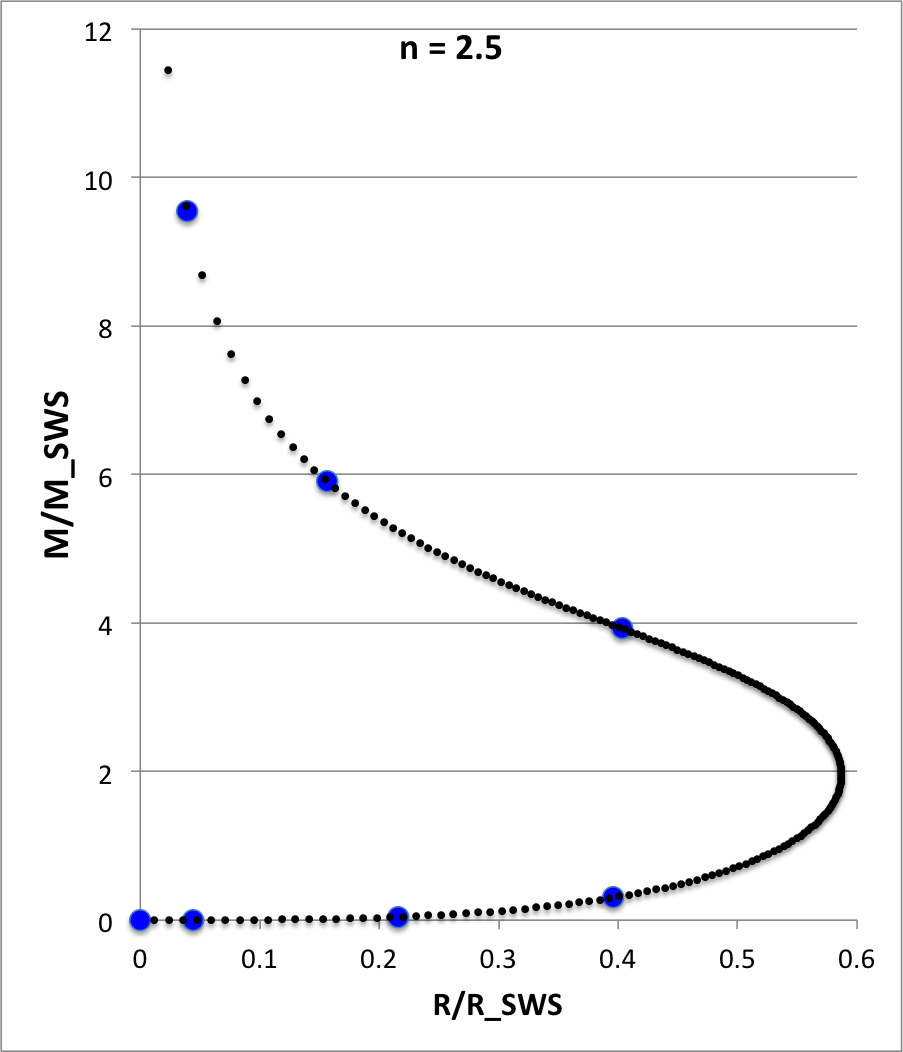
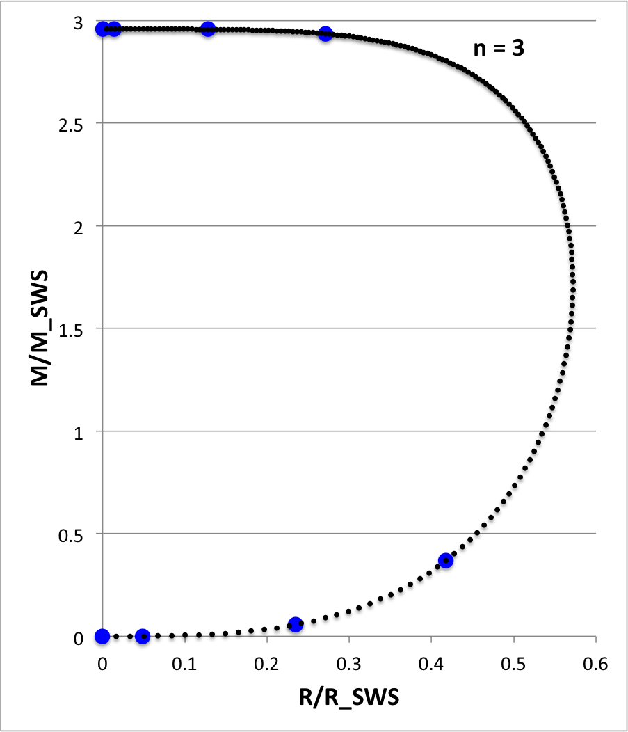
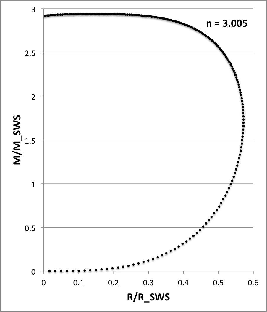
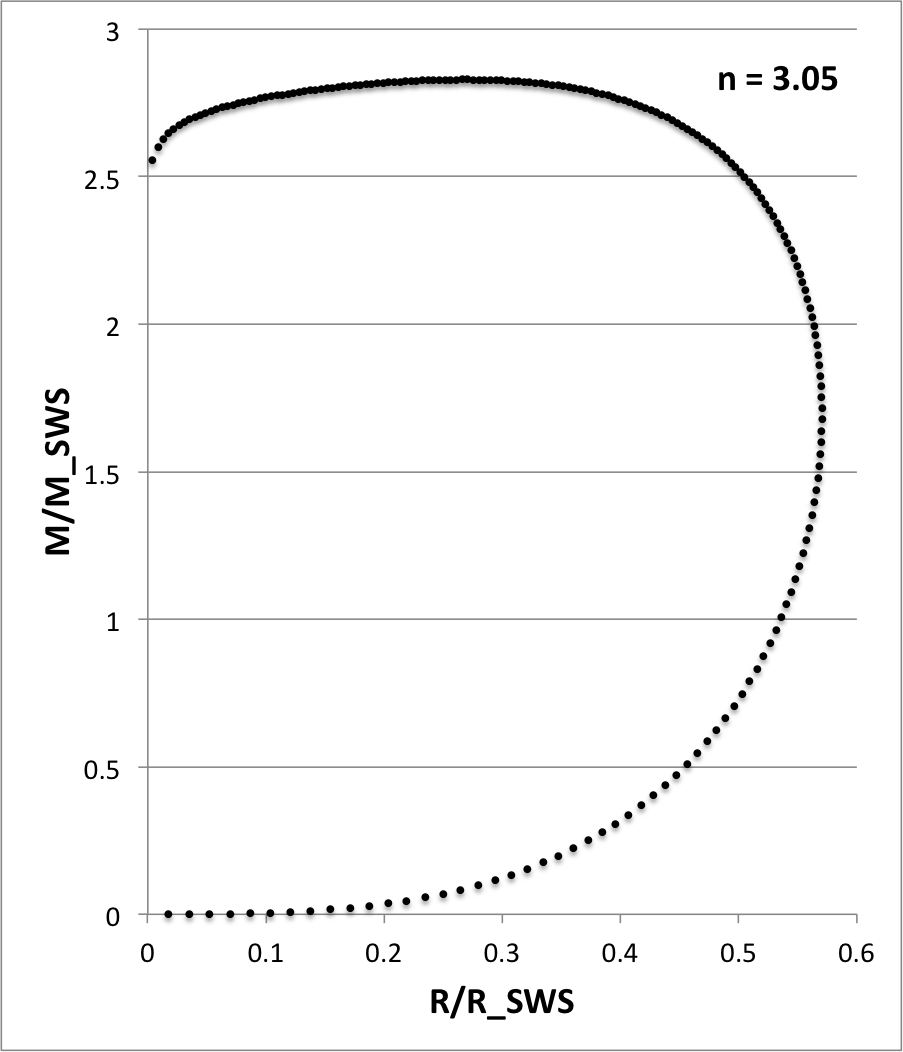
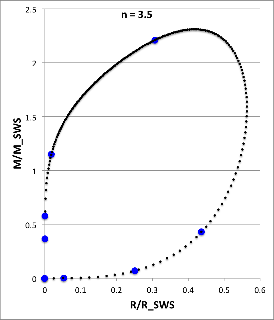
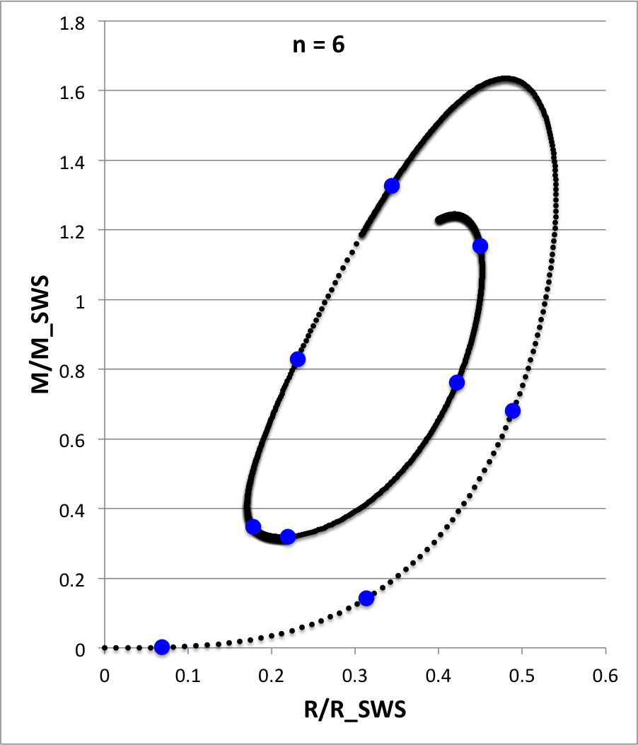
For each of these models, as indicated (n = 2.5, 3, 3.005, 3.05, 3.5, 6), Figure 4 illustrates how the normalized mass, <math>~M/M_\mathrm{SWS}</math>, varies with the normalized radius, <math>~R/R_\mathrm{SWS}</math>, where the definition of these two functions,
|
<math> ~\frac{M}{M_\mathrm{SWS}} </math> |
<math>~\equiv~</math> |
<math> \biggl( \frac{n^3}{4\pi} \biggr)^{1/2} \theta_n^{(n-3)/2} \xi^2 \biggl| \frac{d\theta_n}{d\xi} \biggr| \, , </math> |
|
<math> ~\frac{R}{R_\mathrm{SWS}} </math> |
<math>~\equiv~</math> |
<math> \biggl( \frac{n}{4\pi} \biggr)^{1/2} \xi \theta_n^{(n-1)/2} \, , </math> |
has been drawn from an accompanying discussion of pressure-truncated polytropic configurations. In four of the Figure 4 panels, we have compared the profile of our numerically determined polytropic function (curve defined by <math>~\sim 200</math> small, black circular markers) to results (7 - 9 larger, blue circular markers) taken from Table 2.5.1 of Horedt (2004) — see, specifically the segment of his table on pp. 74 - 75 that applies to polytropic spheres — in an effort to demonstrate that our numerically determined solutions are accurate.
|
Figure 4: Numerically Determined Solutions to the Polytropic Lane-Emden Equation |
||||||||||||||||||||||||||||||||
|---|---|---|---|---|---|---|---|---|---|---|---|---|---|---|---|---|---|---|---|---|---|---|---|---|---|---|---|---|---|---|---|---|
 |
 |
 |
||||||||||||||||||||||||||||||
 |
 |
 |
||||||||||||||||||||||||||||||
|
Data examples from Table 2.5.1 (pp. 74 - 75) of Horedt (2004):
|
||||||||||||||||||||||||||||||||
Emden's (1907) Tabulated Data
| From Table 13 (p. 84) of Emden (1907) — "Global Properties" |
|---|
n xi_1 - theta' 2nd deriv. "mass" rho_c/rho_avg 0 2.4494 0.81647 -0.33333 4.8988 1 0.5 2.7528 0.49975 0.36309 3.7871 1.8361 1 3.14159 0.31831 0.20264 3.14159 3.2899 1.5 3.6571 0.20316 0.11355 2.7176 6.0003 2 4.3518 0.12729 0.06262 2.4107 11.396 2.5 5.4172 0.075 0.02795 2.201 24.076 3 6.9011 0.04231 0.01282 2.015 54.36 4 14.999 0.00803 0.00107 1.8064 623.4 4.5 32.14 0.00168 0.000104 1.7354 6377.7 4.9 169.47 6.04E-05 4.208E-07 1.73554 9.485E+05 5 infinity 0 0 sqrt(3) infinity |
|
The column labeled "mass" contains the tabulated quantity, <math>(-\xi^2 \theta^')_{\xi_1}</math>. |
Horedt's (1986) Tabulated Data
G. P. Horedt (1986), Astrophysics and Space Science, Vol. 126, Issue 2, pp. 357 - 408: Seven-digit tables of Lane-Emden functions
|
In Table I we present seven digit numerical solutions of the Lane-Emden equation for the plane-parallel (N = 1), cylindrical (N = 2), and spherical (N = 3) case for polytropic indices of <math>~n = -10, -5, -4, -3, -2, -1.5, -1.01, -0.9, -0.5, 0, 0.5, 1, 1.5, 2, 3, 4, 5, 6, 10, 20, \pm \infty</math>, supplemented by <math>~n = 2.5, 3.5, 4.5,</math> and <math>~4.99</math> for the spherical case. In Table II some finite boundary values of polytropic slabs, cylinders, and spheres are summarized. For polytropic spheres (N = 3) we have also quoted boundary values near the minimum of the dimensionless mass <math>~-\xi_1^2\theta_1</math>, occurring at n ≈ 4.823 (Z. F. Seidov and R. Kh. Kuzakhmedov, 1978). |
Focusing specifically on the spherically symmetric (N = 3) configurations, we list here the page number(s) on which the table associated with each individual polytropic index can be found in Horedt (1986).
| Spherical (N = 3) Configurations |
||
|---|---|---|
| n | page(s) | <math>~\xi_1</math> |
| - 10 | 386 → 387 | ∞ |
| - 5 | 387 → 388 | ∞ |
| - 4 | 388 → 389 | ∞ |
| - 3 | 389 | ∞ |
| - 2 | 390 | ∞ |
| - 1.5 | 390 → 391 | ∞ |
| - 1.01 | 391 → 392 | ∞ |
| - 0.9 | 392 → 393 | 2.05040073E+00 |
| - 0.5 | 393 | 2.20858842E+00 |
| 0 | 393 → 394 | √6 = 2.44948974E+00 |
| 0.5 | 394 | 2.75269805E+00 |
| 1 | 394 → 395 | π = 3.14159265E+00 |
| 1.5 | 395 | 3.65375374E+00 |
| 2 | 395 → 396 | 4.35287460E+00 |
| 2.5 | 396 → 397 | 5.35527546E+00 |
| 3 | 397 → 398 | 6.89684862E+00 |
| 3.5 | 398 → 399 | 9.53580534E+00 |
| 4 | 399 | 1.49715463E+01 |
| 4.5 | 399 → 400 | 3.18364632E+01 |
| 4.99 | 400 → 401 | 1.75818915+03 |
| 5 | 401 → 402 | ∞ |
| 6 | 402 → 403 | ∞ |
| 10 | 403 → 404 | ∞ |
| 20 | 404 → 405 | ∞ |
| <math>~\pm \infty</math> | 405 → 406 | ∞ |
Related Discussions
- A. T. Service (1977, ApJ 211, 908) — Concise Approximation Formulae for the Lane-Emden Functions

|
|---|
|
© 2014 - 2021 by Joel E. Tohline |

