Radial Oscillations of a Zero-Zero Bipolytrope

This is a chapter that summarizes an accompanying, detailed derivation. A newer version of this chapter, that takes into account a corrected interface matching condition provided by P. Ledoux & Th. Walraven (1958) is provided here.

In a separate chapter on astrophysical interesting equilibrium structures, we have derived analytical expressions that define the equilibrium properties of bipolytropic configurations having <math>~(n_c, n_e) = (0, 0)</math>, that is, bipolytropes in which both the core and the envelope are uniform in density, but the densities in the two regions are different from one another. Letting <math>~R</math> be the radius and <math>~M_\mathrm{tot}</math> be the total mass of the bipolytrope, these configurations are fully defined once any two of the following three key parameters have been specified: The envelope-to-core density ratio, <math>~\rho_e/\rho_c</math>; the radial location of the envelope/core interface, <math>~q \equiv r_i/R</math>; and, the fractional mass that is contained within the core, <math>~\nu \equiv M_\mathrm{core}/M_\mathrm{tot}</math>. These three parameters are related to one another via the expression,

<math>~\frac{q^3}{\nu} \biggl( \frac{1-\nu}{1-q^3} \biggr) \, .</math>

Equilibrium configurations can be constructed that have a wide range of parameter values; specifically,

(We recognize from buoyancy arguments that any configuration in which the envelope density is larger than the core density will be Rayleigh-Taylor unstable, so we restrict our astrophysical discussion to structures for which <math>~\rho_e < \rho_c</math>.)

By employing the linear stability analysis techniques described in an accompanying chapter, we should, in principle, be able to identify a wide range of eigenvectors — that is, radial eigenfunctions and accompanying eigenfrequencies — that are associated with adiabatic radial oscillation modes in any one of these equilibrium, bipolytropic configurations. Using numerical techniques, Murphy & Fiedler (1985), for example, have carried out such an analysis of bipolytropic structures having <math>~(n_c, n_e) = (1,5)</math>. A pair of linear adiabatic wave equations (LAWEs) must be solved — one tuned to accommodate the properties of the core and another tuned to accommodate the properties of the envelope — then the pair of eigenfunctions must be matched smoothly at the radial location of the interface; the identified core- and envelope-eigenfrequencies must simultaneously match.

After identifying the precise form of the LAWEs that apply to the case of <math>~(n_c, n_e) = (0,0)</math> bipolytropes, we discovered that, for a restricted range of key parameters, the pair of equations can both be solved analytically.

Two Separate LAWEs

In an accompanying discussion, we derived the so-called,

Adiabatic Wave (or Radial Pulsation) Equation

<math>~ \frac{d^2x}{dr_0^2} + \biggl[\frac{4}{r_0} - \biggl(\frac{g_0 \rho_0}{P_0}\biggr) \biggr] \frac{dx}{dr_0} + \biggl(\frac{\rho_0}{\gamma_\mathrm{g} P_0} \biggr)\biggl[\omega^2 + (4 - 3\gamma_\mathrm{g})\frac{g_0}{r_0} \biggr] x = 0 </math>

For both regions of the bipolytrope, we define the dimensionless (Lagrangian) radial coordinate,

<math>~\xi \equiv \frac{r_0}{r_i} \, .</math>

So, the interface is, by definition, located at <math>~\xi = 1</math>; and, the surface is necessarily at <math>~\xi = q^{-1}</math>. As the material in the bipolytrope's core (envelope) is compressed/de-compressed during a radial oscillation, we will assume that heating/cooling occurs in a manner prescribed by an adiabat of index <math>~\gamma_c ~(\gamma_e)</math>; in general, <math>~\gamma_e \ne \gamma_c</math>. For convenience, we will also adopt the frequently used shorthand "alpha" notation,

<math>~\alpha_c \equiv 3 - \frac{4}{\gamma_c} \, ,</math> and <math>~\alpha_e \equiv 3 - \frac{4}{\gamma_e} \, .</math>

The Core's LAWE

After adopting, for convenience, the function notation,

<math>~\equiv</math>

<math> 1 + \biggl(\frac{\rho_e}{\rho_c}\biggr) \biggl[ 2 \biggl(1 - \frac{\rho_e}{\rho_c} \biggr) \biggl( 1-q \biggr) + \frac{\rho_e}{\rho_c} \biggl(\frac{1}{q^2} - 1\biggr) \biggr] \, , </math>

we have deduced that, for the core, the LAWE may be written in the form,

<math>~ (1 - \eta^2)\frac{d^2x}{d\eta^2} + ( 4 - 6\eta^2 ) \frac{1}{\eta} \cdot \frac{dx}{d\eta} + \mathfrak{F}_\mathrm{core} x \, . </math>

where,

<math>~\eta \equiv \frac{\xi}{g} \, ,</math> and <math>~\mathfrak{F}_\mathrm{core} \equiv \frac{3\omega_\mathrm{core}^2}{2\pi G\gamma_c \rho_c} - 2\alpha_c\, .</math>

Not surprisingly, this is identical in form to the eigenvalue problem that was first presented — and solved analytically — by Sterne (1937) in connection with his examination of radial oscillations in isolated uniform-density spheres. As is demonstrated below, for the core of our zero-zero bipolytrope, we can in principle adopt any one of the polynomial eigenfunctions and corresponding eigenfrequencies derived by Sterne.

The Envelope's LAWE

Subsequently, we also have deduced that, for the envelope, the governing LAWE becomes,

<math>~ \biggl[ 1 + \frac{(g^2-\mathcal{B}) \xi}{\mathcal{A}} - \mathcal{D} \xi^3\biggr] \frac{d^2x}{d\xi^2} + \biggl\{ 3 + \frac{4(g^2-\mathcal{B}) \xi}{\mathcal{A}} - 6\mathcal{D} \xi^3 \biggr\} \frac{1}{\xi} \cdot \frac{dx}{d\xi} + \biggl[ \mathcal{D} \mathfrak{F}_\mathrm{env} \xi^3 -\alpha_e \biggr]\frac{x}{\xi^2} \, , </math>

where,

<math>~\mathcal{A}</math>	<math>~\equiv</math>	<math>~2\biggl(\frac{\rho_e}{\rho_c}\biggr) \biggl(1 - \frac{\rho_e}{\rho_c} \biggr) \, ; </math>
<math>~\mathcal{B}</math>	<math>~\equiv</math>	<math>~1 + 2\biggl(\frac{\rho_e}{\rho_c}\biggr) - 3\biggl(\frac{\rho_e}{\rho_c}\biggr)^2 \, , </math>
<math>~\mathcal{D}</math>	<math>~\equiv</math>	<math>~\frac{1}{\mathcal{A}}\biggl( \frac{\rho_e}{\rho_c}\biggr)^2 = \biggl[ \frac{\rho_e/\rho_c}{2(1-\rho_e/\rho_c)} \biggr] \, , </math>
<math>~\mathfrak{F}_\mathrm{env}</math>	<math>~\equiv</math>	<math>~\frac{3\omega^2_\mathrm{env}}{2\pi G \gamma_e \rho_e} - 2\alpha_e \, . </math>

We have been unable to demonstrate that this governing equation can be solved analytically for arbitrary pairs of the key model parameters, <math>~q</math> and <math>~\rho_e/\rho_c</math>. But, if we choose parameter value pairs that satisfy the constraint,

<math>~g^2 = \mathcal{B} </math> <math>~\Rightarrow</math> <math>~g = \frac{1}{1+2q^3} \, ,</math> and, <math>~q^3 = \mathcal{D} = \biggl[ \frac{\rho_e/\rho_c}{2(1-\rho_e/\rho_c)} \biggr] </math> <math>~\Rightarrow</math> <math>~\frac{\rho_e}{\rho_c} = \frac{2q^3}{1+2q^3} \, ,</math>

WRONG! The expression that relates <math>~g^2</math> to <math>~q^3</math> should read,

<math>~\frac{1+8q^3}{(1+2q^3)^2} = \frac{1+8\mathcal{D} }{(1+2\mathcal{D})^2}</math>

then the LAWE that is relevant to the envelope simplifies. Specifically, it takes the form,

<math>~0</math>	<math>~=</math>	<math>~ ( 1 - q^3 \xi^3 ) \frac{d^2x}{d\xi^2} + ( 3 - 6q^3 \xi^3 ) \frac{1}{\xi} \cdot \frac{dx}{d\xi} + \biggl[ q^3 \mathfrak{F}_\mathrm{env} \xi^3 -\alpha_e \biggr]\frac{x}{\xi^2} </math>
	<math>~=</math>	<math>~\frac{x}{\xi^2}\biggl\{ ( 1 - q^3 \xi^3 ) \biggl[ \frac{d}{d\ln\xi} \biggl( \frac{d\ln x}{d\ln \xi} \biggr) - \biggl( 1 - \frac{d\ln x}{d\ln \xi} \biggr)\cdot \frac{d\ln x}{d\ln \xi}\biggr] + ( 3 - 6q^3 \xi^3 ) \frac{d\ln x}{d\ln \xi} + \biggl[ q^3 \mathfrak{F}_\mathrm{env} \xi^3 -\alpha_e \biggr] \biggr\} \, . </math>

Shortly after deriving this last expression, we realized that one possible solution is a simple power-law eigenfunction of the form,

where the (constant) exponent is one of the roots of the quadratic equation,

<math>~c_0^2 + 2c_0 - \alpha_e = 0 \, ,</math> <math>~\Rightarrow</math> <math>~c_0 = -1 \pm \sqrt{1+\alpha_e} \, .</math>

This power-law eigenfunction must be paired with the associated, dimensionless eigenfrequency parameter,

<math>~\mathfrak{F}_\mathrm{env}</math>	<math>~=</math>	<math>~c_0(c_0+5) = 3c_0 + \alpha_e</math>
<math>~\Rightarrow ~~~ \frac{3\omega^2_\mathrm{env}}{2\pi G \gamma_e \rho_e} </math>	<math>~=</math>	<math>~ 3(c_0 + \alpha_e) = 3[\alpha_e -1 \pm \sqrt{1+\alpha_e}] \, .</math>

Next, we noticed the strong similarities between the mathematical properties of this eigenvalue problem and the one that was studied by C. Prasad (1948, MNRAS, 108, 414-416) in connection with, what we now recognize to be, a closely related problem. Drawing heavily from Prasad's analysis, we discovered an infinite number of eigenfunctions (each, a truncated polynomial expression) and associated eigenfrequencies that satisfy this governing envelope LAWE. The eigenvectors associated with the lowest few modes are tabulated, below.

Eigenvector

Core Segment

Mode	Core Eigenfunction <math> g^2 \equiv 1 + \biggl(\frac{\rho_e}{\rho_c}\biggr) \biggl[ 2 \biggl(1 - \frac{\rho_e}{\rho_c} \biggr) \biggl( 1-q \biggr) + \frac{\rho_e}{\rho_c} \biggl(\frac{1}{q^2} - 1\biggr) \biggr] </math>	Core Eigenfrequency <math>~\frac{3\omega_\mathrm{core}^2}{2\pi \gamma_c G \rho_c} = 2[\alpha_c + j(2j+5)]</math>
<math>~j=0 </math>	<math>~x_\mathrm{core} = a_0 </math>	<math>~6-8/\gamma_c</math>
<math>~j=1 </math>	<math>~x_\mathrm{core} = a_0 \biggl[ 1 - \frac{7}{5}\biggr(\frac{\xi^2}{g^2}\biggr) \biggr]</math>	<math>~20-8/\gamma_c</math>
<math>~j=2 </math>	<math>~x_\mathrm{core} = a_0 \biggl[ 1 - \frac{18}{5}\biggr(\frac{\xi^2}{g^2}\biggr) + \frac{99}{35}\biggr(\frac{\xi^2}{g^2}\biggr)^2 \biggr]</math>	<math>~42-8/\gamma_c</math>

Envelope Segment

Mode

Envelope Eigenfunction

<math>~c_0 \equiv -1 \pm \sqrt{1+\alpha_e}</math>

Envelope Eigenfrequency

<math>~\frac{3\omega_\mathrm{env}^2}{2\pi \gamma_e G \rho_e} = 3[\alpha_e + c_0(2\ell+1) + \ell(3\ell+5)]</math>

<math>~=2\alpha_e + (c_0+3\ell)(c_0+3\ell + 5)</math>

<math>~x_\mathrm{env} = b_0 \xi^{c_0}</math>

<math>~3[\alpha_e + c_0]</math>

<math>~x_\mathrm{env} = b_0 \xi^{c_0}\biggl\{1 + \biggl[ \frac{c_0(c_0+5)-(c_0+3)(c_0+8)}{(c_0+3)(c_0+5) - \alpha_e} \biggr](q\xi)^3 \biggr\}</math>

<math>~3[\alpha_e + 3c_0 +8]</math>

<math>~x_\mathrm{env} </math>	<math>~=</math>	<math>~b_0 \xi^{c_0}\biggl\{1 + \biggl[ \frac{c_0(c_0+5)-(c_0+6)(c_0+11)}{(c_0+3)(c_0+5) - \alpha_e}\biggr](q\xi)^3 </math>
		<math>~ + \biggl[ \frac{c_0(c_0+5)-(c_0+6)(c_0+11)}{(c_0+3)(c_0+5) - \alpha_e}\biggr]\biggl[ \frac{(c_0+3)(c_0+8)-(c_0+6)(c_0+11)}{(c_0+6)(c_0+8) - \alpha_e}\biggr](q\xi)^6 \biggr\} </math>

<math>~3[\alpha_e + 5c_0 +22]</math>

Piecing Together

Here we illustrate how the two segments of the eigenfunction can be successfully pieced together for the specific case of <math>~(\ell,j) = (2,1)</math>.

STEP 1: Choose a value of the adiabatic exponent for the envelope, <math>~\gamma_e</math>. Then, the values of both <math>~\alpha_e</math> and <math>~c_0</math> are known as well; actually, because it is the root of a quadratic equation, <math>~c_0</math> can, in general, take on one of a pair of values. We will elaborate on this further, below.

STEP 2: Acknowledging that the value of <math>~q</math> has yet to be determined, fix the value of the leading, overall scaling coefficient, <math>~b_0</math>, such that^† <math>~x_\mathrm{env} = 1</math> at the interface, that is, at <math>~\xi = 1</math>. For the case of <math>~\ell=2</math>, this means that, throughout the envelope, the eigenfunction is,

<math>~x_{\ell=2} |_\mathrm{env}</math>

<math>~ \xi^{c_0}\biggl[ \frac{ 1 + q^3 A_{21} \xi^{3} + q^6 A_{21}B_{21}\xi^{6} }{ 1 + q^3 A_{21} + q^6 A_{21}B_{21}}\biggr] \, , </math>

where, the values of the newly introduced coefficients,

<math>~A_{21}</math>	<math>~\equiv</math>	<math>~\biggl[ \frac{c_0(c_0+5) - (c_0 + 6)(c_0 + 11)}{(c_0 + 3)(c_0+5) - \alpha_e}\biggr] \, ,</math>
<math>~B_{21}</math>	<math>~\equiv</math>	<math>~\biggl[ \frac{(c_0+3)(c_0+8) - (c_0 + 6)(c_0 + 11)}{(c_0 + 6)(c_0+8) - \alpha_e}\biggr] \, ,</math>

are also both known.

Wrong expression for <math>~g^2</math>

STEP 3: Recognizing that this segment of the eigenfunction will only satisfy the envelope's LAWE if we restrict our discussion to equilibrium models for which <math>~g^2 = \mathcal{B} = (1+2q^3)^{-1}</math>, we must insert this same restriction on <math>~g^2</math> into the core's eigenfunction. At the same time, we should fix the value of the leading, overall scaling coefficient, <math>~a_0</math>, such that^† <math>~x_\mathrm{core} = 1</math> at the interface <math>~(\xi = 1)</math>. For the case of <math>~j=1</math>, this means that, throughout the core, the eigenfunction is,

<math>~x_{j=1} |_\mathrm{core}</math>

STEP 3: Recognizing that this segment of the eigenfunction will only satisfy the envelope's LAWE if we restrict our discussion to equilibrium models for which <math>~g^2 = \mathcal{B} = [(1+8q^3)/(1+2q^3)^{2}]</math>, we must insert this same restriction on <math>~g^2</math> into the core's eigenfunction. At the same time, we should fix the value of the leading, overall scaling coefficient, <math>~a_0</math>, such that^† <math>~x_\mathrm{core} = 1</math> at the interface <math>~(\xi = 1)</math>. For the case of <math>~j=1</math>, this means that, throughout the core, the eigenfunction is,

<math>~x_{j=1} |_\mathrm{core}</math>

STEP 4: Now we need to ensure that the first derivative with respect to the radial coordinate, <math>~\xi</math>, of both eigenfunction segments match at the interface <math>~(\xi = 1)</math>. Making the notation substitution, <math>~\Chi \equiv q^3</math>, the mathematical relation that accomplishes this is,

<math>~\frac{14(1+2\Chi)^2}{7(1+2\Chi)^2 - 5(1+8\Chi)}</math>	<math>~=</math>	<math>~ \frac{c_0 + (c_0 + 3)A_{21}\Chi + (c_0 + 6)A_{21}B_{21} \Chi^2}{1 + A_{21}\Chi + A_{21}B_{21}\Chi^2} </math>
<math>~\Rightarrow ~~~ 0 </math>	<math>~=</math>	<math>~ [c_0 + (c_0 + 3)A_{21}\Chi + (c_0 + 6)A_{21}B_{21} \Chi^2] [7(1+2\Chi)^2 - 5(1+8\Chi)] - 14(1+2\Chi)^2 [1 + A_{21}\Chi + A_{21}B_{21}\Chi^2] </math>
	<math>~=</math>	<math>~ [c_0 + (c_0 + 3)A_{21}\Chi + (c_0 + 6)A_{21}B_{21} \Chi^2] [2 - 12\Chi + 28\Chi^2 ] - (14 + 56\Chi + 56 \Chi^2) [1 + A_{21}\Chi + A_{21}B_{21}\Chi^2] </math>
	<math>~=</math>	<math>~ 2[c_0 + (c_0 + 3)A_{21}\Chi + (c_0 + 6)A_{21}B_{21} \Chi^2] -12\Chi [c_0 + (c_0 + 3)A_{21}\Chi + (c_0 + 6)A_{21}B_{21} \Chi^2] + 28\Chi^2 [c_0 + (c_0 + 3)A_{21}\Chi + (c_0 + 6)A_{21}B_{21} \Chi^2] </math>
		<math>~ - 14 [1 + A_{21}\Chi + A_{21}B_{21}\Chi^2] - 56\Chi [1 + A_{21}\Chi + A_{21}B_{21}\Chi^2] - 56 \Chi^2 [1 + A_{21}\Chi + A_{21}B_{21}\Chi^2] \, . </math>

Or we have, equivalently,

where,

<math>~e</math>	<math>~\equiv</math>	<math>~ 2c_0 - 14 \, ,</math>
<math>~d</math>	<math>~\equiv</math>	<math>~2(c_0+3)A_{21} - 12c_0 - 14A_{21} - 56</math>
	<math>~=</math>	<math>~2(c_0-4)A_{21} - 4(14 + 3c_0) \, ,</math>
<math>~c</math>	<math>~\equiv</math>	<math>~2(c_0+6)A_{21}B_{21} - 12(c_0+3)A_{21} + 28c_0 - 14A_{21}B_{21} - 56A_{21} - 56 </math>
	<math>~=</math>	<math>~2(c_0 - 1)A_{21}B_{21} - 4(23 + 3c_0)A_{21} + 28(c_0 - 2) \, ,</math>
<math>~b</math>	<math>~\equiv</math>	<math>~-12(c_0+6)A_{21}B_{21} + 28(c_0+3)A_{21} - 56A_{21}B_{21} - 56A_{21} </math>
	<math>~=</math>	<math>~- 4(3c_0+32)A_{21}B_{21} + 28(c_0+1)A_{21} \, ,</math>
<math>~a</math>	<math>~\equiv</math>	<math>~28(c_0+4)A_{21}B_{21} \, .</math>

Wrong expressions for quadratic equation coefficients, based on previous, wrong expression for <math>~g^2</math>

<math>~e</math>	<math>~\equiv</math>	<math>~ 14- 2c_0 \, ,</math>
<math>~d</math>	<math>~\equiv</math>	<math>~28(2-c_0) + (8-2c_0) A_{21} \, ,</math>
<math>~c</math>	<math>~\equiv</math>	<math>~28(2-c_0) - 28(1+c_0) A_{21} + 2(1 - c_0)A_{21}B_{21} \, ,</math>
<math>~b</math>	<math>~\equiv</math>	<math>~-28A_{21}[(1+c_0) + (4+c_0)B_{21} ] \, ,</math>
<math>~a</math>	<math>~\equiv</math>	<math>~- 28 (4+c_0)A_{21}\cdot B_{21} \, .</math>

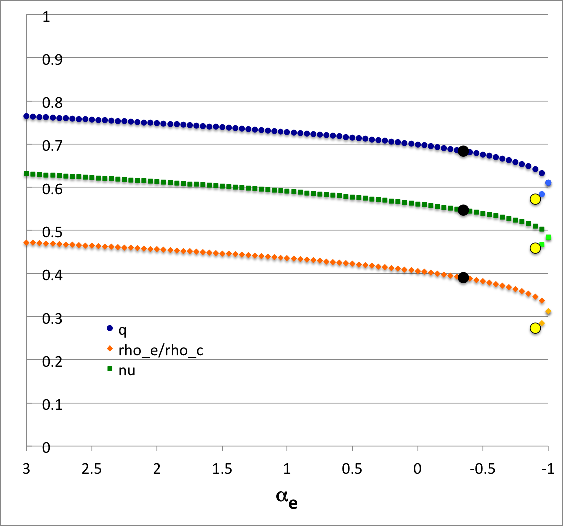
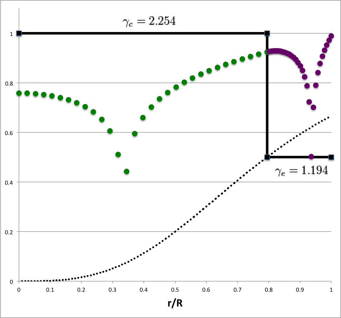
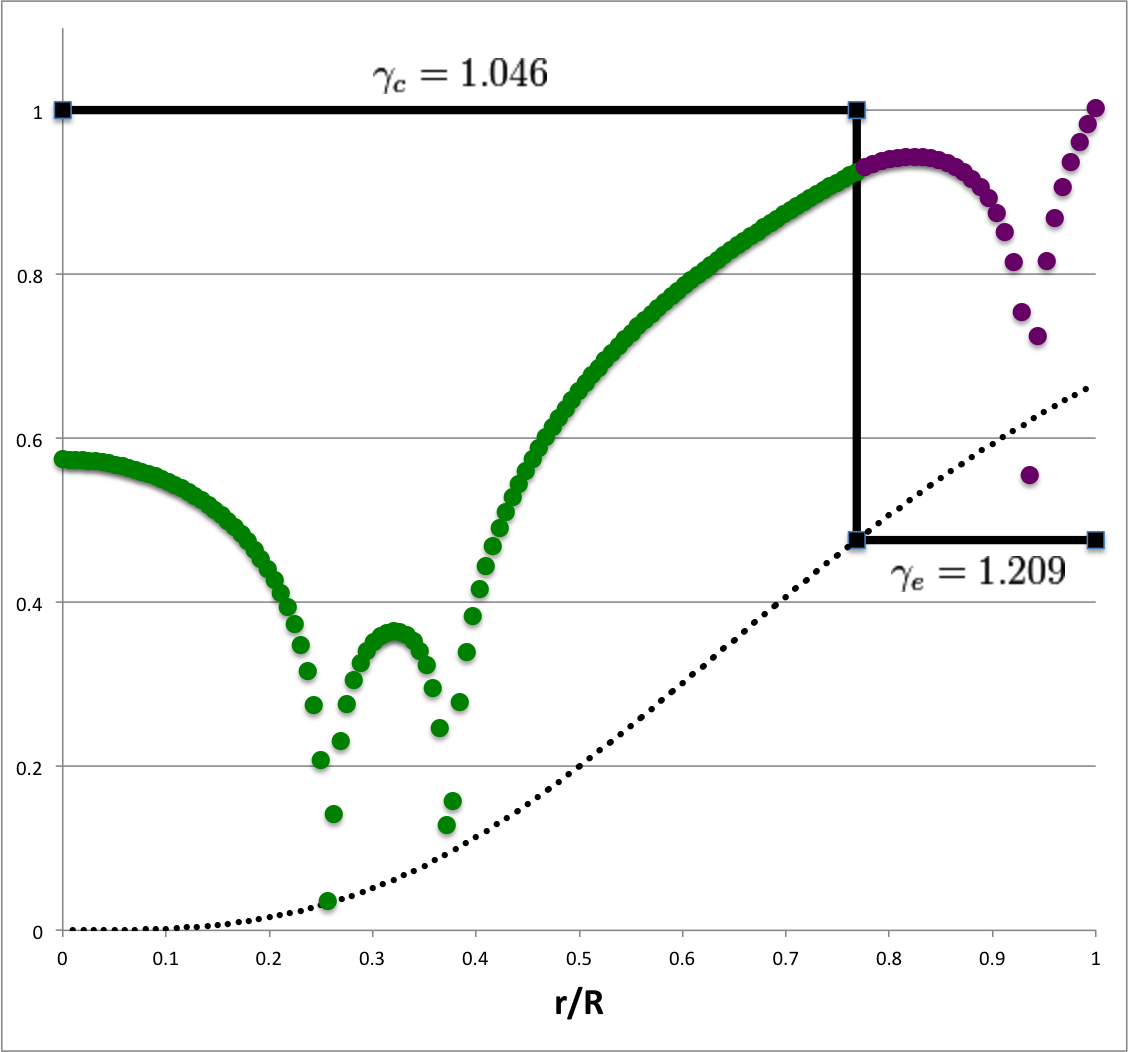
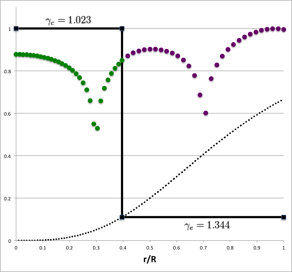
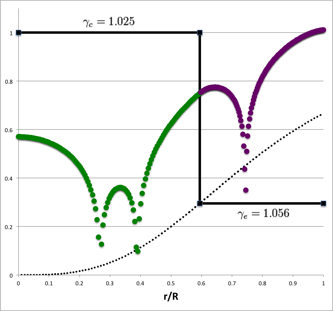
The physically relevant (real) root of this quartic equation in <math>~\Chi</math> — see our accompanying detailed presentation — gives us the specific value of the dimensionless interface location, <math>~q</math>, for which both the values and the first derivatives of the two eigenfunction segments match at the interface. As is shown by the plot displayed in the right-hand panel of Figure 1, we have found different values of <math>~q</math> for each choice (STEP 1) of <math>~\gamma_e</math> (or, equivalently, choice of <math>~\alpha_e</math>). In this plot we have purposely flipped the horizontal axis so that the extreme left <math>~(\alpha_e = +3)</math> represents an incompressible <math>~(n = 0)</math> envelope, while the extreme right represents an isothermal <math>~(\gamma_e = 1)</math> envelope.

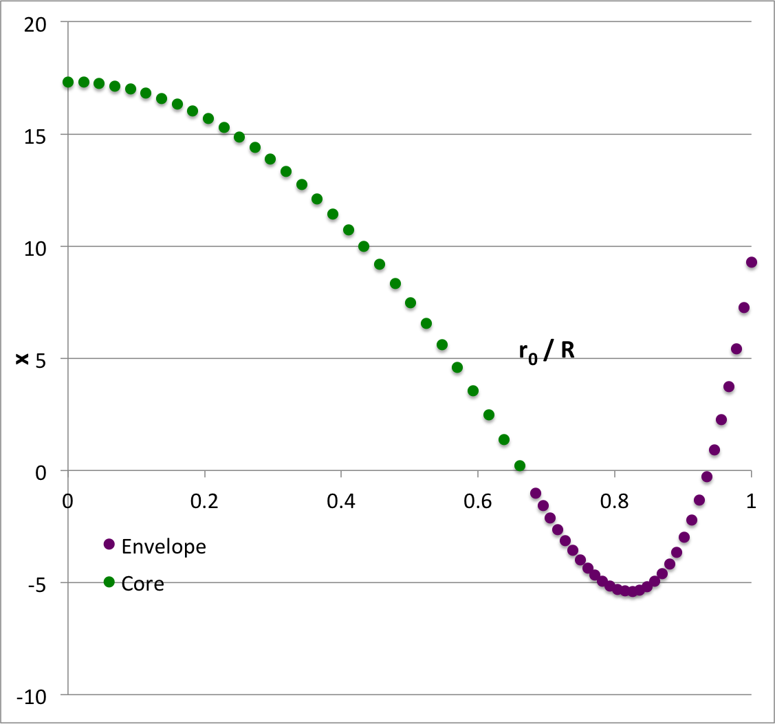
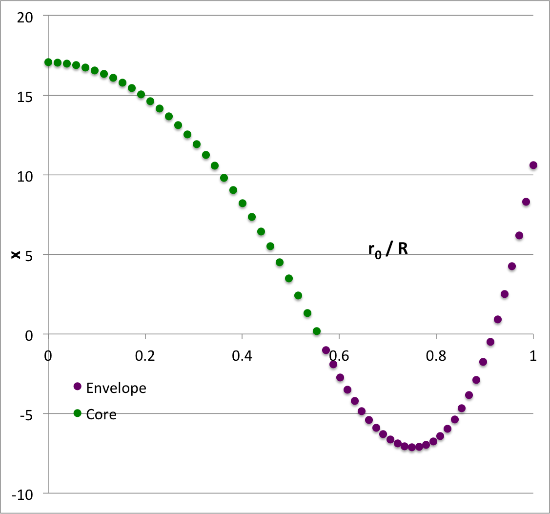
Figure 1

<math>~\alpha_e = -0.35 \, ;~~~c_0 = \sqrt{1+\alpha_e} - 1</math>

Directly Above: Plot shows for which equilibrium bipolytropic configurations with <math>~(n_c, n_e) = (0,0)</math> we are able to construct analytically prescribed eigenvectors for the radial oscillation mode, <math>~(\ell, j) = (2,1)</math>. The top (blue), middle (green), and bottom (orange) curves show how <math>~q</math>, <math>~\nu</math>, and <math>~\rho_e/\rho_c</math> vary with the specified value of the envelope's adiabatic exponent over the full, physically reasonable range of the parameter, <math>~-1 \le \alpha_e \le 3</math>. For the upper portion of each curve (dark blue, dark green, dark orange), the parameter, <math>~c_0</math>, is taken to be the "plus" root of its defining quadratic equation; the "minus" root defines <math>~c_0</math> along the lower portion of each curve (light blue, light green, light orange).

Upper-left Quadrant: An <math>~x(r_0/R)</math> plot showing the radial structure of the analytically prescribed eigenfunction for <math>~\alpha_e = -0.35</math> and <math>~c_0</math> (plus); its underlying, equilibrium model characteristics are identified by the black circular marker in the above plot.

Lower-left Quadrant: The analytcially prescribed eigenfunction, <math>~x(r_0/R)</math>, for <math>~\alpha_e = -0.9</math> and <math>~c_0</math> (minus); its underlying, equilibrium model characteristics are identified by the yellow circular marker in the above plot.

^†Note that, as displayed here, the sign has been flipped on both <math>~x(r_0/R)</math> eigenfunctions so that, in practice, the amplitude at the interface is negative one, rather than positive one. Plotted in this way, we immediately recognize that both eigenfunctions are qualitatively similar to the <math>~j = 2</math> radial oscillation eigenfunction that was derived by Sterne (1937) in the context of isolated, homogeneous spheres.

<math>~c_0</math> (plus):

<math>~\gamma_e</math>:

<math>~n_e</math>:

<math>~q</math>:

<math>~\nu</math>:

<math>~\rho_e/\rho_c</math>:

<math>~\alpha_c</math>:

<math>~\gamma_c</math>:

<math>~\alpha_e = -0.9 \, ;~~~c_0 = -\sqrt{1+\alpha_e} - 1</math>

<math>~c_0</math> (minus):

<math>~\gamma_e</math>:

<math>~n_e</math>:

<math>~q</math>:

<math>~\nu</math>:

<math>~\rho_e/\rho_c</math>:

<math>~\alpha_c</math>:

<math>~\gamma_c</math>:

STEP 5: Finally, for each choice of <math>~\gamma_e</math> — or, alternatively, <math>~\alpha_e</math> — the physically relevant value of the core's adiabatic exponent is set by demanding that the dimensional eigenfrequencies of the envelope and core precisely match. That is, we demand that,

Figure 2

<math>~\omega^2_\mathrm{env} = \omega^2_\mathrm{core} \, .</math>

From above, we know that, for the core,

<math>~3\omega^2_\mathrm{core}\biggr|_\mathrm{j=1} = 2\pi \gamma_c G \rho_c [ 20 - 8/\gamma_c] \, ;</math>

whereas, for the envelope,

<math>~3\omega^2_\mathrm{env}\biggr|_\mathrm{\ell=2} = 2\pi \gamma_e G \rho_e [ 3(\alpha_e + 5c_0 + 22)] \, .</math>

By demanding that these frequencies be identical, we conclude that,

<math>~ \gamma_c </math>

<math>~\frac{1}{20} \biggl[ 8 + 3\gamma_e \biggl(\frac{\rho_e}{\rho_c}\biggr) \biggl(\alpha_e + 5c_0 + 22 \biggr)\biggr] \, .</math>

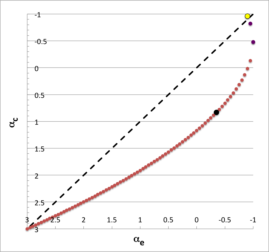
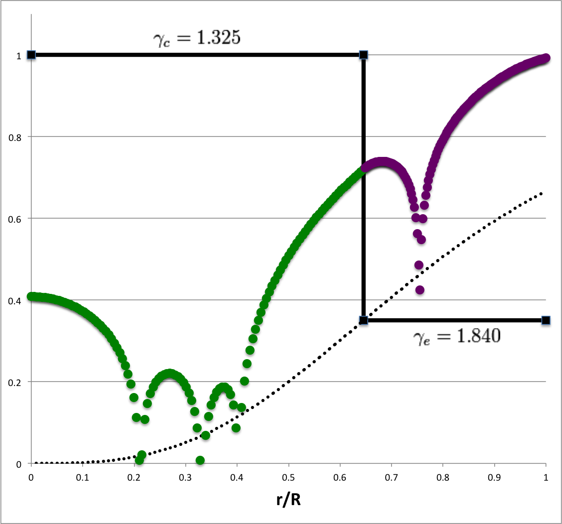
Figure 2 shows how the required value of <math>~\alpha_c</math> varies with the choice of <math>~\alpha_e</math>; here, both axes have been flipped in order to run from incompressible <math>~(\alpha = +3)</math> at the left/bottom, to isothermal <math>~(\alpha = -1)</math> at the right/top. For the lower portion of the curve (red circular markers), the parameter, <math>~c_0</math>, is taken to be the "plus" root of its defining quadratic equation; the "minus" root defines <math>~c_0</math> along the upper portion of the curve (purple circular markers). The diagonal dashed-black line identifies where <math>~\alpha_c = \alpha_e</math>; in models below and to the right of this line, the envelope is more compressible than is the core, whereas in models above and to the left of this line, the core is more compressible than the envelope.

The eigenfrequency that corresponds to the specific eigenfunction that is displayed in upper-left quadrant of Figure 1 is identified by the black circular marker in Figure 2; as is indicated by the row of numbers on the left in Figure 1, this model has,

<math>~\gamma_c = 1.845579 </math> <math>~\Rightarrow </math> <math>~\alpha_c = +0.8326535 \, . </math>

The yellow circular marker in Figure 2 identifies the model whose analytically prescribed, <math>~(\ell,j) = (2,1)</math> eigenfunction is displayed in the lower-left quadrant of Figure 1; it has,

<math>~\gamma_c = 1.0102231 </math> <math>~\Rightarrow </math> <math>~\alpha_c = -0.9595214 \, . </math>

Examining Alignment with Surface Boundary Condition

Expectation

As we have reviewed in an accompanying discussion, one astrophysically reasonable surface boundary condition provides a mathematical relationship between the logarithmic derivative of the eigenfunction with respect to the radius, in terms of the eigenfrequency as follows:

<math>~ \frac{d\ln x}{d\ln \xi}\biggr\|_{\xi = 1/q}</math>	<math>~=</math>	<math>~\frac{3\omega^2 }{4\pi G\rho_c \gamma_e} \biggl( \frac{\nu}{q^3}\biggr) - \biggl( 3 - \frac{4}{\gamma_e}\biggr) </math>
	<math>~=</math>	<math>~\frac{3\omega^2 }{4\pi G\rho_c \gamma_e} \biggl( \frac{1+2q^3}{3q^3}\biggr) - \alpha_e </math>
	<math>~=</math>	<math>~\frac{1}{3} \biggl[\frac{3\omega^2 }{2\pi G\rho_c \gamma_e} \biggr] \biggl( \frac{\rho_c}{\rho_e}\biggr) - \alpha_e </math>
	<math>~=</math>	<math>~\frac{1}{3} \biggl[\mathfrak{F}_\mathrm{env} + 2\alpha_e \biggr] - \alpha_e </math>
	<math>~=</math>	<math>~\frac{1}{3} \biggl[\mathfrak{F}_\mathrm{env} - \alpha_e \biggr] \, . </math>

Now, according to our above-described envelope segment of the eigenfunction, we established the analytic prescription,

<math>~\mathfrak{F}_\mathrm{env}</math>

in which case the desired surface boundary condition is,

<math>~ 3 \cdot \frac{d\ln x}{d\ln \xi}\biggr\|_{\xi = 1/q}</math>	<math>~=</math>	<math>~ (c_0 + 3\ell)(c_0 + 3\ell+5) - \alpha_e </math>
	<math>~=</math>	<math>~ [c_0^2 + c_0(6\ell + 5 ) + 3\ell(3\ell+5)] - (c_0^2 + 2c_0)</math>
	<math>~=</math>	<math>~ 3[ c_0(2\ell + 1 ) + \ell(3\ell+5)]</math>

That is, we expect to find the following,

Desired Boundary Condition
<math>~\frac{d\ln x}{d\ln \xi}\biggr\|_{\xi = 1/q}</math>	<math>~=</math>	<math>~ c_0(2\ell + 1 ) + \ell(3\ell+5) \, .</math>

Analytic2

Continuing, from above, a discussion specifically of the case, <math>~\ell = 2</math>, the analytically specified envelope eigenfunction is,

<math>~x_{\ell=2} |_\mathrm{env}</math>

<math>~ \xi^{c_0}\biggl[ \frac{ 1 + q^3 A_{\ell=2} \xi^{3} + q^6 A_{\ell=2}B_{\ell=2}\xi^{6} }{ 1 + q^3 A_{\ell=2} + q^6 A_{\ell=2}B_{\ell=2}}\biggr] \, , </math>

where, the values of the newly introduced coefficients,

<math>~A_{\ell=2}</math>	<math>~\equiv</math>	<math>~\biggl[ \frac{c_0(c_0+5) - (c_0 + 6)(c_0 + 11)}{(c_0 + 3)(c_0+5) - \alpha_e}\biggr] = \frac{-2(2c_0+11)}{(2c_0+5)} \, ,</math>
<math>~B_{\ell=2}</math>	<math>~\equiv</math>	<math>~\biggl[ \frac{(c_0+3)(c_0+8) - (c_0 + 6)(c_0 + 11)}{(c_0 + 6)(c_0+8) - \alpha_e}\biggr] = \frac{-(c_0+7)}{2(c_0+4)} \, ,</math>

in which case,

<math>~\frac{d\ln x}{d\ln \xi} = \frac{\xi}{x} \cdot \frac{dx}{d\xi} \biggl\|_\mathrm{env}</math>	<math>~=</math>	<math>~\frac{\xi}{x} \biggl\{ c_0\xi^{c_0-1}\biggl[ \frac{ 1 + q^3 A \xi^{3} + q^6 AB\xi^{6} }{ 1 + q^3 A + q^6 AB}\biggr] + \xi^{c_0}\biggl[ \frac{ 3q^3 A \xi^{2} + 6q^6 AB\xi^{5} }{ 1 + q^3 A + q^6 AB}\biggr] \biggr\} </math>
	<math>~=</math>	<math>~ c_0 + \biggl[ \frac{ 3q^3 A \xi^{3} + 6q^6 AB\xi^{6} }{ 1 + q^3 A\xi^3 + q^6 AB\xi^6}\biggr] \, . </math>

Hence, at the surface <math>~(\xi = 1/q)</math>, we find,

<math>~\frac{d\ln x}{d\ln \xi} \biggl\|_{\xi=1/q}</math>	<math>~=</math>	<math>~ c_0 +\biggl[ \frac{ 3 A + 6 AB }{ 1 + A + AB}\biggr] </math>
	<math>~=</math>	<math>~ c_0 +\biggl[ \frac{ -12(2c_0+11)(c_0+4) + 12(2c_0+11)(c_0+7) }{ 2(2c_0 + 5)(c_0+4) - 4(2c_0+11)(c_0+4) + 2(2c_0+11) (c_0+7)}\biggr] </math>
	<math>~=</math>	<math>~ c_0 +6\biggl[ \frac{ (2c_0^2 + 25c_0 + 77) -(2c_0^2 + 19c_0 +44) }{ (2c_0^2 + 13c_0 + 20) - 2(2c_0^2 + 19c_0 + 44) + (2c_0^2 + 25c_0 + 77)}\biggr] </math>
	<math>~=</math>	<math>~ c_0 +6 \biggl[ \frac{ 6c_0 +33 }{ 9}\biggr] </math>
	<math>~=</math>	<math>~ 5c_0 + 22 \, . </math>

It is gratifying — although, somewhat surprising (to me!) — to find that this precisely matches the above-defined, desired boundary condition for the case of <math>~\ell = 2</math>.

Duh!

After also checking conformance with the expected boundary condition in the case of analytic eigenfunctions having <math>~\ell = 3</math> and, separately (not shown), for numerically generated eigenfunctions having a wide range of oscillation frequencies, it dawned on us that the "desired" surface boundary condition may actually be a natural outcome of the envelope's LAWE.

By constraining our discussion to models for which <math>~g^2 = \mathcal{B}</math> and <math>~\mathcal{D} = q^3</math>, the envelope's LAWE is,

<math>~ \biggl[ 1 - q^3 \xi^3\biggr] \frac{d^2x}{d\xi^2} + \biggl\{ 3 - 6q^3 \xi^3 \biggr\} \frac{1}{\xi} \cdot \frac{dx}{d\xi} + \biggl[ q^3 \mathfrak{F}_\mathrm{env} \xi^3 -\alpha_e \biggr]\frac{x}{\xi^2} \, . </math>

At the surface <math>~(\xi = 1/q)</math>, the coefficient of the second derivative term goes to zero, in which case the LAWE reduces in form to,

<math>~0</math>	<math>~=</math>	<math>~ -\frac{3}{\xi} \cdot \frac{dx}{d\xi} + \biggl[ \mathfrak{F}_\mathrm{env} -\alpha_e \biggr]\frac{x}{\xi^2} </math>
<math>~\Rightarrow ~~~ 3\cdot \frac{d\ln x}{d\ln \xi}\biggr\|_\mathrm{surface} </math>	<math>~=</math>	<math>~ \mathfrak{F}_\mathrm{env} -\alpha_e \, . </math>

And this is precisely the condition that derives from the astrophysically reasonable boundary condition that we have discussed separately and that has been reviewed, above.

Broader Analysis

Let's, then, examine the behavior of the envelope's LAWE at the surface in the most general case — that is, when not constrained to <math>~g^2 = \mathcal{B}</math>. First, we note that,

<math>~g^2 - \mathcal{B}</math>	<math>~=</math>	<math> \biggl(\frac{\rho_e}{\rho_c}\biggr) \biggl[ 2 \biggl(1 - \frac{\rho_e}{\rho_c} \biggr) \biggl( 1-q \biggr) + \frac{\rho_e}{\rho_c} \biggl(\frac{1}{q^2} - 1\biggr) \biggr] -2\biggl(\frac{\rho_e}{\rho_c}\biggr) + 3\biggl(\frac{\rho_e}{\rho_c}\biggr)^2 </math>
	<math>~=</math>	<math> \biggl(\frac{\rho_e}{\rho_c}\biggr) \biggl\{ 2 \biggl[1 - \biggl(\frac{\rho_e}{\rho_c} \biggr) -q + q \biggl(\frac{\rho_e}{\rho_c} \biggr)\biggr] + \biggl( \frac{\rho_e}{\rho_c} \biggr)\frac{1}{q^2} -2 + 2\biggl(\frac{\rho_e}{\rho_c}\biggr) \biggr\} </math>
	<math>~=</math>	<math> \biggl(\frac{\rho_e}{\rho_c}\biggr) \biggl[ - 2q + 2q \biggl(\frac{\rho_e}{\rho_c} \biggr) + \biggl( \frac{\rho_e}{\rho_c} \biggr)\frac{1}{q^2} \biggr] </math>
	<math>~=</math>	<math> \frac{1}{q^2} \biggl(\frac{\rho_e}{\rho_c}\biggr) \biggl[ \biggl( \frac{\rho_e}{\rho_c} \biggr) + 2q^3 \biggl(\frac{\rho_e}{\rho_c} - 1 \biggr) \biggr] \, . </math>

Hence, at the surface quite generally, the coefficient of the second derivative is,

<math>~\frac{1}{\mathcal{A}}\biggl[\mathcal{A} + (g^2 - \mathcal{B})\xi - \mathcal{A}\mathcal{D} \xi^3 \biggr]_{\xi=1/q}</math>	<math>~=</math>	<math>~ \frac{1}{\mathcal{A}}\biggl\{ 2\biggl(\frac{\rho_e}{\rho_c}\biggr) \biggl(1-\frac{\rho_e}{\rho_c}\biggr) + \frac{1}{q^3} \biggl(\frac{\rho_e}{\rho_c}\biggr) \biggl[ \biggl( \frac{\rho_e}{\rho_c} \biggr) + 2q^3 \biggl(\frac{\rho_e}{\rho_c} - 1 \biggr) \biggr] - \frac{1}{q^3}\biggl(\frac{\rho_e}{\rho_c}\biggr)^2 \biggr\} </math>
	<math>~=</math>	<math>~ \frac{1}{\mathcal{A}} \biggl(\frac{\rho_e}{\rho_c}\biggr)\biggl\{ - 2\biggl(\frac{\rho_e}{\rho_c} -1\biggr) + \frac{1}{q^3} \biggl[ \biggl( \frac{\rho_e}{\rho_c} \biggr) + 2q^3 \biggl(\frac{\rho_e}{\rho_c} - 1 \biggr) \biggr] - \frac{1}{q^3}\biggl(\frac{\rho_e}{\rho_c}\biggr) \biggr\} </math>
	<math>~=</math>	<math>~ 0 \, . </math>

And, at the surface quite generally, the coefficient of the first derivative is,

<math>~\frac{1}{\mathcal{A}}\biggl[3\mathcal{A} + 4(g^2 - \mathcal{B})\xi - 6\mathcal{A}\mathcal{D} \xi^3 \biggr]_{\xi=1/q}</math>	<math>~=</math>	<math>~ \frac{1}{\mathcal{A}}\biggl\{ 6\biggl(\frac{\rho_e}{\rho_c}\biggr) \biggl(1-\frac{\rho_e}{\rho_c}\biggr) + \frac{4}{q^3} \biggl(\frac{\rho_e}{\rho_c}\biggr) \biggl[ \biggl( \frac{\rho_e}{\rho_c} \biggr) + 2q^3 \biggl(\frac{\rho_e}{\rho_c} - 1 \biggr) \biggr] - \frac{6}{q^3}\biggl(\frac{\rho_e}{\rho_c}\biggr)^2 \biggr\} </math>
	<math>~=</math>	<math>~ \frac{2}{\mathcal{A}} \biggl(\frac{\rho_e}{\rho_c}\biggr) \biggl\{ -3\biggl(\frac{\rho_e}{\rho_c} - 1\biggr) + \frac{2}{q^3} \biggl[ \biggl( \frac{\rho_e}{\rho_c} \biggr) + 2q^3 \biggl(\frac{\rho_e}{\rho_c} - 1 \biggr) \biggr] - \frac{3}{q^3}\biggl(\frac{\rho_e}{\rho_c}\biggr) \biggr\} </math>
	<math>~=</math>	<math>~ \frac{2}{\mathcal{A}} \biggl(\frac{\rho_e}{\rho_c}\biggr) \biggl[ \biggl(\frac{\rho_e}{\rho_c} - 1\biggr) - \frac{1}{q^3}\biggl(\frac{\rho_e}{\rho_c}\biggr) \biggr] \, . </math>

Hence, at the surface quite generally, the envelope's LAWE becomes,

<math>~ - \biggl[ 3\mathcal{A} + 4(g^2-\mathcal{B}) \xi - 6\mathcal{A} \mathcal{D} \xi^3 \biggr]_{\xi=1/q} \frac{d\ln x}{d\ln\xi} \biggr\|_\mathrm{surface} </math>	<math>~=</math>	<math>~ \mathcal{A}\biggl[ \mathcal{D} \mathfrak{F}_\mathrm{env} \xi^3 -\alpha_e \biggr]_{\xi=1/q} </math>
<math>~\Rightarrow~~~ - 2\biggl(\frac{\rho_e}{\rho_c}\biggr) \biggl[ \biggl(\frac{\rho_e}{\rho_c} - 1\biggr) - \frac{1}{q^3}\biggl(\frac{\rho_e}{\rho_c}\biggr) \biggr] \frac{d\ln x}{d\ln\xi} \biggr\|_\mathrm{surface} </math>	<math>~=</math>	<math>~ \biggl(\frac{\rho_e}{\rho_c}\biggr)^2 \mathfrak{F}_\mathrm{env} \cdot \frac{1}{q^3} - 2\alpha_e \biggl(\frac{\rho_e}{\rho_c}\biggr)\biggl(1- \frac{\rho_e}{\rho_c}\biggr) </math>
<math>~\Rightarrow~~~ \biggl[2\biggl(\frac{\rho_e}{\rho_c}\biggr) + 2q^3\biggl(1 - \frac{\rho_e}{\rho_c} \biggr) \biggr] \frac{d\ln x}{d\ln\xi} \biggr\|_\mathrm{surface} </math>	<math>~=</math>	<math>~ \biggl(\frac{\rho_e}{\rho_c}\biggr) \mathfrak{F}_\mathrm{env} - 2q^3 \alpha_e \biggl(1- \frac{\rho_e}{\rho_c}\biggr) </math>
<math>~\Rightarrow~~~ \frac{d\ln x}{d\ln\xi} \biggr\|_\mathrm{surface} </math>	<math>~=</math>	<math>~\biggl[2 + 2q^3\biggl(1 - \frac{\rho_e}{\rho_c} \biggr)\biggl(\frac{\rho_e}{\rho_c}\biggr)^{-1} \biggr] ^{-1} \biggl[ \mathfrak{F}_\mathrm{env} - 2q^3 \alpha_e \biggl(1- \frac{\rho_e}{\rho_c}\biggr)\biggl(\frac{\rho_e}{\rho_c}\biggr)^{-1} \biggr] </math>
	<math>~=</math>	<math>~ \frac{\mathfrak{F}_\mathrm{env} - \Kappa \alpha_e}{2+\Kappa} \, , </math>

where,

<math>~\Kappa \equiv 2q^3\biggl(1 - \frac{\rho_e}{\rho_c} \biggr)\biggl(\frac{\rho_e}{\rho_c}\biggr)^{-1} \, .</math>

Notice that in the special case for which we have been able to identify analytically specifiable eigenvectors, namely, when

<math>~g^2 = \mathcal{B} </math> <math>~\Rightarrow</math> <math>~\Kappa = 1 \, ,</math>

this surface boundary condition simplifies to the expected expression,

<math>~ \frac{d\ln x}{d\ln\xi} \biggr|_\mathrm{surface} </math>

<math>~\frac{1}{3} \biggl[ \mathfrak{F}_\mathrm{env} - \alpha_e \biggr] \, . </math>

Under what condition — other than when <math>~g^2=\mathcal{B}</math> — does the general expression generate the expected expression? We need,

<math>~\frac{1}{3} \biggl[ \mathfrak{F}_\mathrm{env} - \alpha_e \biggr] </math>	<math>~=</math>	<math>~\biggl[2 + \Kappa \biggr] ^{-1} \biggl[ \mathfrak{F}_\mathrm{env} - \alpha_e \Kappa \biggr] </math>
<math>~\Rightarrow ~~~ (2 + \Kappa ) \biggl[ \mathfrak{F}_\mathrm{env} - \alpha_e \biggr] </math>	<math>~=</math>	<math>~ 3\biggl[ \mathfrak{F}_\mathrm{env} - \alpha_e \Kappa \biggr] </math>
<math>~\Rightarrow ~~~ (2 + \Kappa ) \mathfrak{F}_\mathrm{env} - (2 + \Kappa ) \alpha_e </math>	<math>~=</math>	<math>~ 3\mathfrak{F}_\mathrm{env} - 3\Kappa \alpha_e </math>
<math>~\Rightarrow ~~~ (\Kappa -1) \mathfrak{F}_\mathrm{env} </math>	<math>~=</math>	<math>~ -2(\Kappa-1 ) \alpha_e </math>
<math>~\Rightarrow ~~~ \mathfrak{F}_\mathrm{env} </math>	<math>~=</math>	<math>~ -2\alpha_e \, . </math>

But, given that,

<math>~\mathfrak{F}_\mathrm{env}</math>

<math>~\equiv</math>

<math>~\frac{3\omega^2_\mathrm{env}}{2\pi G \gamma_e \rho_e} - 2\alpha_e \, , </math>

we see that the expected boundary condition will result only for <math>~\omega_\mathrm{env}^2 = 0</math>, that is, only for, <math>~\sigma_c^2 = 0</math>. This is what we have been noticing as we have played with numerically generated eigenvectors: When integrating from the center of the zero-zero bipolytrope, to its surface, the naturally resulting (first) derivative of the eigenfunction at the surface of the configuration matches the expected surface boundary condition …

for all values of <math>\sigma_c^2</math>, when <math>~g^2= \mathcal{B}</math>, that is, when <math>~\Kappa=1</math>;
only for <math>~\sigma_c^2 = 0</math> in all other configurations, that is, for all <math>~\Kappa \ne 1</math>.

What do we make of this?

Five Mode Summary

<math>~(\ell, j) = (2,1)</math>	<math>~(\ell, j) = (2,2)</math>

<math>~\frac{3\omega^2}{2\pi G\rho_c} = 37.08874</math> more details …	<math>~\frac{3\omega^2}{2\pi G\rho_c} = 35.95210</math> more details …

<math>~(\ell, j) = (3,1)</math>	<math>~(\ell, j) = (3,2)</math>	<math>~(\ell, j) = (3,3)</math>

<math>~\frac{3\omega^2}{2\pi G\rho_c} = 12.452545</math> more details …	<math>~\frac{3\omega^2}{2\pi G\rho_c} = 35.05461</math> more details …	<math>~\frac{3\omega^2}{2\pi G\rho_c} = 87.41594</math> more details …

Model	<math>~\ell</math>	<math>~j</math>	<math>~q</math>	<math>~\gamma_e</math>	<math>~\gamma_c</math>	<math>~\nu</math>	<math>~\frac{\rho_e}{\rho_c}</math>	<math>~\alpha_e</math>	<math>~\alpha_c</math>	<math>~n_e</math>	<math>~n_c</math>	<math>~g^2</math>	<math>~f</math>	<math>~\sigma_\mathfrak{G}^2</math>	Analytic <math>~\sigma_c^2</math>
Analytic21	2	1	0.684	1.194	1.846	0.547	0.390	-0.35	+0.833	5.15	1.18	1.324	2.542	+0.761	28.9116
Analytic22	2	2	0.887	1.799	1.022	0.799	0.583	+0.776	-0.914	1.25	46	1.146	1.444	-0.878	34.9155
Analytic31	3	1	0.406	1.180	1.009	0.378	0.118	-0.390	-0.964	5.56	111	1.194	3.568	-0.180	12.1770
Analytic32	3	2	0.812	2.327	4.216	0.690	0.517	+1.281	+2.051	0.754	0.311	1.232	1.813	+9.654	169.0733

<math>~\sigma_c^2</math> Determined from Numerical Integration by Enforcing Boundary Condition (B.C.) <math>\frac{d \ln x_\mathrm{env}}{d\ln \xi}\biggr\|_\mathrm{surface} = c_0(2\ell+1) + \ell(3\ell+5)</math>
Model	<math>~\ell=0</math> B.C.: <math>~c_0</math>	<math>~\ell=1</math> B.C.: <math>~(3c_0+8)</math>	<math>~\ell=2</math> B.C.: <math>~(5c_0+22)</math>	<math>~\ell=3</math> B.C.: <math>~7(c_0+6)</math>	<math>~\ell=4</math> B.C.: <math>~(9c_0+68)</math>
Analytic21	-0.76017962	+9.881793	+28.9116	+56.32919	-
Analytic22	-4.890477	+5.5864115	+34.91550	+83.09678	-

Broad Application

Here's one key lesson that can be drawn from our analytically specified oscillation modes. As has been documented above, the quantum number, <math>~j</math>, associated with the eigenvector of the core is related to the oscillation frequency,

<math>~\sigma_c^2</math>

<math>~\equiv</math>

<math>~\frac{3\omega^2}{2\pi G \rho_c} \, ,</math>

via the expression,

<math>~\frac{\sigma_c^2}{\gamma_c} - 2\alpha_c</math>	<math>~=</math>	<math>~ 2j(2j+5) </math>
<math>~\Rightarrow~~~\sigma_c^2</math>	<math>~=</math>	<math>~\frac{8[\alpha_c + j(2j+5)]}{3-\alpha_c} \, .</math>

Also, as documented above, the quantum number, <math>~\ell</math>, associated with the eigenvector of the envelope is related to the oscillation frequency via the expression,

<math>~\frac{\sigma_c^2}{\gamma_e(\rho_e/\rho_c)} - 2\alpha_e</math>	<math>~=</math>	<math>~(c_0 + 3\ell)(c_0 + 3\ell + 5) </math>
<math>~\Rightarrow~~~\sigma_c^2</math>	<math>~=</math>	<math>~\gamma_e \biggl(\frac{\rho_e}{\rho_c}\biggr) \biggl[2\alpha_e + (c_0 + 3\ell)(c_0 + 3\ell + 5) \biggr]</math>
	<math>~=</math>	<math>~\biggl(\frac{\rho_e}{\rho_c}\biggr) \frac{4[2c_0^2 + 4c_0 + c_0^2 + c_0(6\ell+5) + 3\ell(3\ell+5) ]}{3-\alpha_e}</math>
	<math>~=</math>	<math>~\biggl(\frac{\rho_e}{\rho_c}\biggr) \frac{12[c_0^2 + c_0(2\ell+3) + \ell(3\ell+5) ]}{3-\alpha_e} \, ,</math>

$Comment by J. E. Tohline on 4 February 2017: This expression for the density ratio is a necessary but not sufficient relationship. According to each analytic solution, once the pair of quantum numbers <math>~(\ell,j)</math> has been specified, the two adiabatic indexes cannot be specified independently of one another.$

where, as a reminder, <math>~c_0 = [-1 \pm \sqrt{1+\alpha_e}]</math>. Eliminating <math>~\sigma_c^2</math> between these two relations gives,

<math>~\frac{\rho_e}{\rho_c}</math>	<math>~=</math>	<math>~\frac{2(3-\alpha_e) [\alpha_c + j(2j+5)]}{3(3-\alpha_c) [c_0^2 + c_0(2\ell+3) + \ell(3\ell+5) ]} </math>
	<math>~=</math>	<math>~\frac{(3-\alpha_e) \sigma_c^2}{12 [c_0^2 + c_0(2\ell+3) + \ell(3\ell+5) ]} \, .</math>

Case A

Consider, first, the astrophysical system in which <math>~(n_c, n_e) = (5, 1)</math>. Given that, in general, <math>~\alpha = (3-n)/(1+n)</math>, we therefore will be considering the system in which, <math>~(\alpha_c, \alpha_e) = (-\tfrac{1}{3}, 1) </math>. For this system, we should be able to analytically specify eigenvectors having the properties specified in the following table.

Analytically Specifiable Eigenvectors for which <math>~(n_c, n_e) = (5, 1)</math> <math>~\Rightarrow</math> <math>~(\alpha_c, \alpha_e) = (-\tfrac{1}{3}, 1)</math>
		<math>~\frac{\rho_e}{\rho_c}</math>
<math>~\ell</math>	<math>~c_0</math>	<math>~j=1</math> <math>~(\sigma_c^2 = 16)</math>	<math>~j=2</math> <math>~(\sigma_c^2 = 42.4)</math>
1	<math>~-1 + \sqrt{2}</math>	0.26034953	n/a <math>~(q > 1)</math>
1	<math>~-1 - \sqrt{2}</math>	1.52 (n/a)	(n/a)
2	<math>~-1 + \sqrt{2}</math>	0.10636430	0.28186540
2	<math>~-1 - \sqrt{2}</math>	0.24400066	0.64660175
3	<math>~-1 + \sqrt{2}</math>	0.05809795	0.15395957
3	<math>~-1 - \sqrt{2}</math>	0.10216916	0.27074827

Related Discussions

User:Tohline/SSC/Stability/BiPolytrope0 0Old

Contents

Radial Oscillations of a Zero-Zero Bipolytrope

Two Separate LAWEs

The Core's LAWE

The Envelope's LAWE

Eigenvector

Core Segment

Envelope Segment

Piecing Together

Examining Alignment with Surface Boundary Condition

Expectation

Analytic2

Duh!

Broader Analysis

Five Mode Summary

Broad Application

Case A

Related Discussions

Navigation menu

Search