Difference between revisions of "User:Tohline/Apps/WoodwardTohlineHachisu94"
| (21 intermediate revisions by the same user not shown) | |||
| Line 1: | Line 1: | ||
__FORCETOC__ | |||
<!-- __NOTOC__ will force TOC off --> | |||
=The Stability of Self-Gravitating Polytropic Tori= | =The Stability of Self-Gravitating Polytropic Tori= | ||
| Line 4: | Line 6: | ||
[[Image:LSU_Structure_still.gif|74px|left]] | [[Image:LSU_Structure_still.gif|74px|left]] | ||
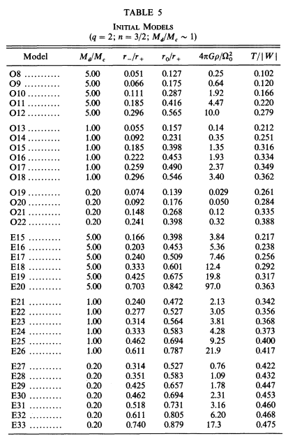
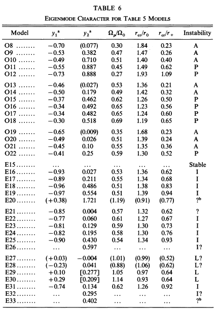
[http://adsabs.harvard.edu/abs/1994ApJ...420..247W J. W. Woodward, J. E. Tohline, & I. Hachisu] (1994; hereafter WTH94) used nonlinear numerical hydrodynamic techniques to examine the relative stability of self-gravitating, polytropic tori toward the development of nonaxisymmetric structure. | [http://adsabs.harvard.edu/abs/1994ApJ...420..247W J. W. Woodward, J. E. Tohline, & I. Hachisu] (1994; hereafter WTH94) used nonlinear numerical hydrodynamic techniques to examine the relative stability of self-gravitating, polytropic tori toward the development of nonaxisymmetric structure. The following pair of tables list key properties of the set of model tori that were examined: Table 5 gives characteristics of the initial models and Table 6 presents results ascertained from the numerical stability analyses. | ||
<div align="center"> | <div align="center"> | ||
<table border="1" cellpadding="5"> | <table border="1" cellpadding="5"> | ||
<tr><td align="center"> | <tr><td align="center" colspan="2"> | ||
Table extracted from [http://adsabs.harvard.edu/abs/1994ApJ...420..247W J. W. Woodward, J. E. Tohline & I. Hachisu (1994)]<p></p> | Table extracted from [http://adsabs.harvard.edu/abs/1994ApJ...420..247W J. W. Woodward, J. E. Tohline & I. Hachisu (1994)]<p></p> | ||
"''The Stability of Thick, Self-gravitating Disks in Protostellar Systems''"<p></p> | "''The Stability of Thick, Self-gravitating Disks in Protostellar Systems''"<p></p> | ||
| Line 17: | Line 17: | ||
<tr> | <tr> | ||
<td> | <td> | ||
[[File:WTH94_Table5.png| | [[File:WTH94_Table5.png|350px|center|Woodward, Tohline & Hachisu (1994, ApJ, 420, 247)]] | ||
</td> | |||
<td><p></p> | |||
[[File:WTH94_Table6.png|360px|center|Woodward, Tohline & Hachisu (1994, ApJ, 420, 247)]] | |||
</td> | </td> | ||
</tr> | </tr> | ||
</table> | </table> | ||
</div> | </div> | ||
==Adopted Notation== | |||
This subsection has been drawn from an [[User:Tohline/Appendix/Ramblings/Azimuthal_Distortions#Adopted_Notation|accompanying discussion]] that details how the linear-amplitude development of nonaxisymmetric structure is often analyzed in numerical simulations. | |||
Beginning with equation (2) of [http://adsabs.harvard.edu/abs/1990ApJ...361..394T TH90] but ignoring variations in the vertical coordinate direction, the mass density is given by the expression, | |||
<div align="center"> | |||
<table border="0" cellpadding="5" align="center"> | |||
<tr> | |||
<td align="right"> | |||
<math>~\rho</math> | |||
</td> | |||
<td align="center"> | |||
<math>~=</math> | |||
</td> | |||
<td align="left"> | |||
<math>~\rho_0 \biggl[ 1 + f(\varpi)e^{-i(\omega t - m\phi)} \biggr] \, ,</math> | |||
</td> | |||
</tr> | |||
</table> | |||
</div> | |||
where it is understood that <math>~\rho_0</math>, which defines the structure of the initial axisymmetric equilibrium configuration, is generally a function of the cylindrical radial coordinate, <math>~\varpi</math>. | |||
Using the subscript, <math>~m</math>, to identify the time-invariant coefficients and functions that characterize the intrinsic eigenvector of each azimuthal eigen-mode, and acknowledging that the associated eigenfrequency will in general be imaginary, that is, | |||
<div align="center"> | |||
<table border="0" cellpadding="5" align="center"> | |||
<tr> | |||
<td align="right"> | |||
<math>~\omega_m</math> | |||
</td> | |||
<td align="center"> | |||
<math>~=</math> | |||
</td> | |||
<td align="left"> | |||
<math>~\omega_R + i\omega_I \, ,</math> | |||
</td> | |||
</tr> | |||
</table> | |||
</div> | |||
we expect each unstable mode to display the following behavior: | |||
<div align="center"> | |||
<table border="0" cellpadding="5" align="center"> | |||
<tr> | |||
<td align="right"> | |||
<math>~\biggl[ \frac{\rho}{\rho_0} - 1 \biggr]</math> | |||
</td> | |||
<td align="center"> | |||
<math>~=</math> | |||
</td> | |||
<td align="left"> | |||
<math>~f_m(\varpi)e^{-i[\omega_R t + i \omega_I t - m\phi_m(\varpi)]} </math> | |||
</td> | |||
</tr> | |||
<tr> | |||
<td align="right"> | |||
| |||
</td> | |||
<td align="center"> | |||
<math>~=</math> | |||
</td> | |||
<td align="left"> | |||
<math>~\biggl\{ f_m(\varpi)e^{-im\phi_m(\varpi)}\biggr\} e^{-i\omega_R t } \cdot e^{\omega_I t} </math> | |||
</td> | |||
</tr> | |||
<tr> | |||
<td align="right"> | |||
| |||
</td> | |||
<td align="center"> | |||
<math>~=</math> | |||
</td> | |||
<td align="left"> | |||
<math>~\biggl\{ f_m(\varpi)e^{-i[\omega_R t + m\phi_m(\varpi)]} \biggr\} e^{\omega_I t} \, .</math> | |||
</td> | |||
</tr> | |||
</table> | |||
</div> | |||
Adopting [http://adsabs.harvard.edu/abs/1986PThPh..75..251K Kojima's (1986)] notation, that is, defining, | |||
<div align="center"> | |||
<table border="0" cellpadding="5" align="center"> | |||
<tr> | |||
<td align="right"> | |||
<math>~y_1 \equiv \frac{\omega_R}{\Omega_0} - m</math> | |||
</td> | |||
<td align="center"> | |||
and | |||
</td> | |||
<td align="left"> | |||
<math>~y_2 \equiv \frac{\omega_I}{\Omega_0} \, ,</math> | |||
</td> | |||
</tr> | |||
</table> | |||
</div> | |||
the eigenvector's behavior can furthermore be described by the expression, | |||
<div align="center"> | |||
<table border="0" cellpadding="5" align="center"> | |||
<tr> | |||
<td align="right"> | |||
<math>~\biggl[ \frac{\rho}{\rho_0} - 1 \biggr]</math> | |||
</td> | |||
<td align="center"> | |||
<math>~=</math> | |||
</td> | |||
<td align="left"> | |||
<math>~\biggl\{ f_m(\varpi)e^{-i[(y_1+m) (\Omega_0 t) + m\phi_m(\varpi)]} \biggr\} e^{y_2 (\Omega_0 t)} </math> | |||
</td> | |||
</tr> | |||
<tr> | |||
<td align="right"> | |||
| |||
</td> | |||
<td align="center"> | |||
<math>~=</math> | |||
</td> | |||
<td align="left"> | |||
<math>~\biggl\{ f_m(\varpi)e^{-im[(y_1/m+1) (\Omega_0 t) + \phi_m(\varpi)]} \biggr\} e^{y_2 (\Omega_0 t)} \, .</math> | |||
</td> | |||
</tr> | |||
</table> | |||
</div> | |||
Note that, as viewed from a frame of reference that is rotating with the mode pattern frequency, | |||
<div align="center"> | |||
<math>\Omega_p \equiv \frac{\omega_R}{m} = \Omega_0\biggl(\frac{y_1}{m}+1\biggr) \, ,</math> | |||
</div> | |||
we should find an eigenvector of the form, | |||
<div align="center"> | |||
<table border="0" cellpadding="5" align="center"> | |||
<tr> | |||
<td align="right"> | |||
<math>~\biggl[ \frac{\delta\rho}{\rho_0}\biggr]_\mathrm{rot} \equiv \biggl[ \frac{\rho}{\rho_0} - 1 \biggr]e^{im\Omega_p t}</math> | |||
</td> | |||
<td align="center"> | |||
<math>~=</math> | |||
</td> | |||
<td align="left"> | |||
<math>~\biggl\{ f_m(\varpi)e^{-im[\phi_m(\varpi)]} \biggr\} e^{y_2 (\Omega_0 t)} \, ,</math> | |||
</td> | |||
</tr> | |||
</table> | |||
</div> | |||
whose relative amplitude — with a radial structure as specified inside the curly braces — is undergoing a uniform exponential growth but is otherwise unchanging. | |||
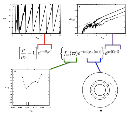
Drawing from figure 2 of [http://adsabs.harvard.edu/abs/1994ApJ...420..247W WTH94], our Figure 1, immediately below, illustrates how the behavior of each factor in this expression can reveal itself during a numerical simulation that follows the time-evolutionary development of an unstable, nonaxisymmetric eigenmode. The initial model for this depicted evolution (model O3 from Table 1 of [http://adsabs.harvard.edu/abs/1994ApJ...420..247W WTH94]) is a zero-mass — that is, it is a [[User:Tohline/Apps/PapaloizouPringleTori#Massless_Polytropic_Tori|Papaloizou-Pringle like torus]] — with [[User:Tohline/SR#Barotropic_Structure|polytropic index]],<math>~n = 3</math>, and a rotation-law profile defined by [[User:Tohline/AxisymmetricConfigurations/SolutionStrategies#Simple_Rotation_Profile_and_Centrifugal_Potential|uniform specific angular momentum]]. | |||
* The top-left panel shows how, at any radial location, the phase angle, <math>~\phi_1/(2\pi)</math>, for the <math>~m=1</math> eigenmode, varies with time, <math>~t/t_\mathrm{rot}</math>, where, <math>~t_\mathrm{rot} \equiv 2\pi/\Omega_0</math> is the rotation period at the density maximum; | |||
* Using a semi-log plot, the top-right panel shows the exponential growth of the amplitude of three separate modes: The dominant unstable mode, displaying the largest amplitude, is <math>~m = 1</math>. | |||
* Using a semi-log plot (log amplitude versus fractional radius, <math>~\varpi/r_+</math>), the bottom-left panel displays the shape of the eigenfunction, <math>~f_1(\varpi)</math>, for the unstable, <math>~m=1</math> mode; | |||
* The bottom-right panel displays the radial dependence of the equatorial-plane phase angle, <math>~\phi_1(\varpi)</math>, for the unstable, <math>~m=1</math> mode; this is what [http://adsabs.harvard.edu/abs/2011Ap%26SS.334....1H HI11] refer to as the "constant phase locus." | |||
<div align="center" id="Figure1"> | |||
<table border="1" cellpadding="5" width="70%"> | |||
<tr> | |||
<td align="center"> | |||
<b><font size="+1">Figure 1</font></b> | |||
</td> | |||
</tr> | |||
<tr><td align="center"> | |||
Four panels extracted<sup>†</sup> from figure 2, p. 252 of [http://adsabs.harvard.edu/abs/1994ApJ...420..247W J. W. Woodward, J. E. Tohline & I. Hachisu (1994)]<p></p> | |||
"''The Stability of Thick, Self-gravitating Disks in Protostellar Systems''"<p></p> | |||
ApJ, vol. 420, pp. 247-267 © [http://aas.org/ American Astronomical Society] | |||
</td></tr> | |||
<tr> | |||
<td align="center"> | |||
[[File:Diagram01.png|550px|Rearranged Figure 2 from Woodward, Tohline, and Hachisu (1994)]] | |||
</td> | |||
</tr> | |||
<tr><td align="left"><sup>†</sup>As displayed here, the layout of figure panels (a, b, c, d) has been modified from the original publication layout; otherwise, each panel is unmodified.</td></tr> | |||
</table> | |||
</div> | |||
==Online Movies== | ==Online Movies== | ||
<table border="1" cellpadding="8" align="center" width=" | Drawing from the description presented in §Va of [http://adsabs.harvard.edu/abs/1994ApJ...420..247W WTH94], the early evolution of each model behaved qualitatively in a manner depicted in Figure 1, above. For the first few rotation periods, the amplitude remained quite small for all azimuthal Fourier modes — see early times in the upper-right panel of Figure 1 — and there was no apparent organized behavior exhibited by the Fourier phase angles, <math>~\phi_m</math>. Then a clearly identifiable eigenfunction for either mode <math>~m = 1</math> or <math>~m = 2</math> developed out of the initially random noise, signaled by an exponential growth of the mode amplitude — see late times in the upper-right panel of Figure 1 — and a periodic oscillation of <math>~\phi_m</math> — see late times in the upper-left panel of Figure 1. A clear depiction of the radially dependent (bottom-left figure panel) ''and'' azimuthally dependent (bottom-right figure panel) structure of the unstable mode also emerged from the initially random noise. The bottom-right panel of Figure 1 displays, specifically for the [http://adsabs.harvard.edu/abs/1994ApJ...420..247W WTH94] model '''O3''' the ''constant phase locus'' that was present at late times. | ||
<table border="1" cellpadding="8" align="center" width="80%"> | |||
<tr> | <tr> | ||
<th align="center" colspan="3"><font size="+1">Figure | <th align="center" colspan="3"><font size="+1">Figure 2:</font> | ||
Animation Sequences to Supplement | Animation Sequences to Supplement Figure 10 of [http://adsabs.harvard.edu/abs/1994ApJ...420..247W WTH94]<p></p> | ||
(click on security-lock icon or caption model name to go to YouTube)</th> | (click on security-lock icon or caption model name to go to YouTube)</th> | ||
</tr> | </tr> | ||
<tr> | <tr> | ||
<td align="center" bgcolor="black"> | <td align="center" bgcolor="black"> | ||
[https://youtu.be/ | [https://youtu.be/ASaKuIJfs3c [[File:Model_O15.png|200px|Click for YouTube Video]] ] | ||
</td> | </td> | ||
<td align="center" rowspan="4">[[File:WTH94Fig10.png|350px|Figure 10 from WTH94]] | |||
<td align="center" bgcolor="black"> | <td align="center" bgcolor="black"> | ||
[https://youtu.be/kif3ClH6YAs [[File:Model_O14.png|200px|Click for YouTube Video]] ] | [https://youtu.be/kif3ClH6YAs [[File:Model_O14.png|200px|Click for YouTube Video]] ] | ||
</td> | </td> | ||
</tr> | </tr> | ||
<tr> | <tr> | ||
<td align="center">[https://youtu.be/ | <td align="center">[https://youtu.be/ASaKuIJfs3c Table 5, Model O15]</td> | ||
<td align="center">[https://youtu.be/kif3ClH6YAs Table 5, Model O14]</td> | <td align="center">[https://youtu.be/kif3ClH6YAs Table 5, Model O14]</td> | ||
</tr> | </tr> | ||
<tr> | <tr> | ||
<td align="center" bgcolor="black"> | <td align="center" bgcolor="black"> | ||
[https://youtu.be/ | [https://youtu.be/t0iqCmbjsNk [[File:Model_E17.png|200px|Click for YouTube Video]] ] | ||
</td> | </td> | ||
<td align="center" bgcolor="black"> | <td align="center" bgcolor="black"> | ||
[https://youtu.be/ | [https://youtu.be/6s3DMd7yXiA [[File:Model_E29.png|200px|Click for YouTube Video]] ] | ||
</td> | </td> | ||
<td align="center" | </tr> | ||
[https://youtu.be/ | <tr> | ||
<td align="center">[https://youtu.be/t0iqCmbjsNk Table 5, Model E17]</td> | |||
<td align="center">[https://youtu.be/6s3DMd7yXiA Table 5, Model E29]</td> | |||
</tr> | |||
<tr> | |||
<td align="left" colspan="3"> | |||
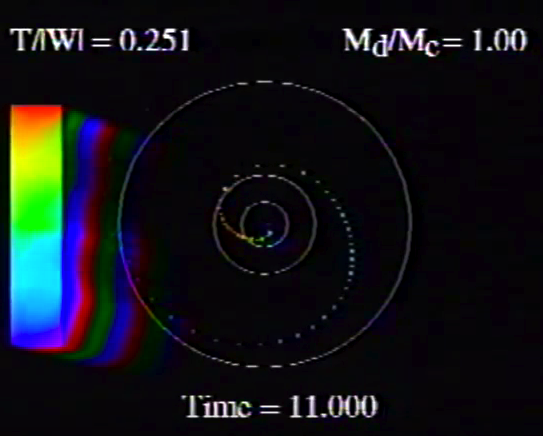
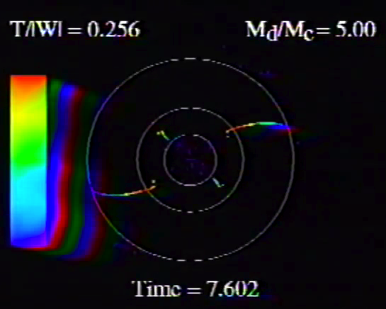
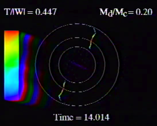
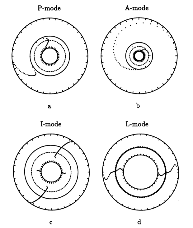
Caption to Fig. 10 from [http://adsabs.harvard.edu/abs/1994ApJ...420..247W WTH94]: ''Constant phase locus'' diagrams — that is, "<math>~\phi_m - r</math>" diagrams — illustrating the azimuthal structure of the four specific eigenmodes that were found to be dynamically unstable in our modeled disks. ''(a)'' The ''m = 1'' P-mode, shown here as it developed in model '''O15''' <math>~[M_d/M_c = 1; ~T/|W| = 0.316];</math> ''(b)'' The ''m = 1'' A-mode, shown here as it developed in model '''O14''' <math>~[M_d/M_c = 1; ~T/|W| = 0.251];</math> ''(c)'' The ''m = 2'' I-mode, shown here as it developed in model '''E17''' <math>~[M_d/M_c = 5; ~T/|W| = 0.256];</math> ''(d)'' The ''m = 2'' L-mode, shown here as it developed in model '''E29''' <math>~[M_d/M_c = 0.2; ~T/|W| = 0.447]\, .</math> | |||
</td> | </td> | ||
</tr> | </tr> | ||
</table> | |||
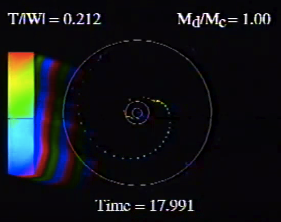
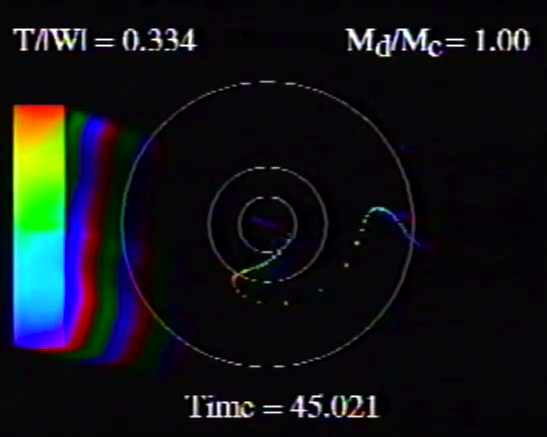
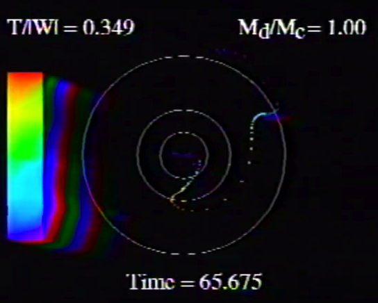
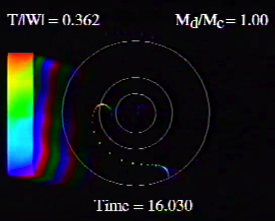
The middle panel of our Figure 2 is a reproduction of Figure 10 from [http://adsabs.harvard.edu/abs/1994ApJ...420..247W WTH94]. It shows the ''constant phase locus'' that emerged from the noise at late times during the evolution of four models: (a) Model '''O15'''; (b) model '''O14'''; (c) model '''E17'''; and (d) model '''E29'''. In the early '90s when this set of model simulations was carried out, we saved numerical data that detailed the time-evolutionary behavior of both the radial and azimuthal structure of each model's fastest growing eigenfunction. This data allowed us to generate after-the-fact, for example, plots of the ''constant phase locus'' at many different points in time to explicitly show how the azimuthally dependent eigenfunction developed out of the initial noise. Using techniques described in [https://www.computer.org/csdl/magazine/cs/2007/06/mcs2007060076/13rRUNvyaoN Tohline (2007)], we transferred these plots, frame by frame, to VHS video tape so that this development could be viewed as an animation. Recently we have employed an analog-to-digital converter to create digital animations from nine of these analog VHS recordings, and each of the animations has been uploaded to YouTube. (The result of these analog-to-digital conversions was, unfortunately, digital animations of low fidelity. They are nevertheless informative.) Our Figure 2 displays a still image from, and provides a link to the YouTube animations that depict the time-evolutionary behavior of models '''O15''' (upper left), '''O14''' (upper right), '''E17''' (lower left), and '''E29''' (lower right); in order to play the desired YouTube video, click on the security-lock icon or the model name that accompanies the associated still image. | |||
Links to five additional animation sequences are provided, immediately below, in our Figure 3. As is identified by the short caption accompanying each still image, these animations are from, respectively, models '''O13''', '''O16''', '''O17''', '''O18''', and '''O22'''. | |||
<table border="1" cellpadding="8" align="center"> | |||
<tr> | <tr> | ||
< | <th align="center" colspan="5"><font size="+1">Figure 3:</font> | ||
Five Additional Animation Sequences to Supplement Table 5 of [http://adsabs.harvard.edu/abs/1994ApJ...420..247W WTH94]<p></p> | |||
(click on security-lock icon or caption model name to go to YouTube)</th> | |||
</tr> | </tr> | ||
<tr> | <tr> | ||
<td align="center" bgcolor="black"> | <td align="center" bgcolor="black"> | ||
[https://youtu.be/ | [https://youtu.be/pcfmvIptn8c [[File:Model_O13.png|200px|Click for YouTube Video]] ] | ||
</td> | |||
<td align="center" bgcolor="black"> | |||
[https://youtu.be/WSJlHlfT_IM [[File:Model_O16.png|200px|Click for YouTube Video]] ] | |||
</td> | |||
<td align="center" bgcolor="black"> | |||
[https://youtu.be/TygfP8-Dc-M [[File:Model_O17.png|200px|Click for YouTube Video]] ] | |||
</td> | </td> | ||
<td align="center" bgcolor="black"> | <td align="center" bgcolor="black"> | ||
[https://youtu.be/ | [https://youtu.be/FGwXtce1R0w [[File:Model_O18.png|200px|Click for YouTube Video]] ] | ||
</td> | </td> | ||
<td align="center" bgcolor="black"> | <td align="center" bgcolor="black"> | ||
[https://youtu.be/ | [https://youtu.be/TKkOhdTQrww [[File:Model_O22.png|200px|Click for YouTube Video]] ] | ||
</td> | </td> | ||
</tr> | </tr> | ||
<tr> | <tr> | ||
<td align="center">[https://youtu.be/pcfmvIptn8c Table 5, Model O13]</td> | |||
<td align="center">[https://youtu.be/WSJlHlfT_IM Table 5, Model O16]</td> | |||
<td align="center">[https://youtu.be/TygfP8-Dc-M Table 5, Model O17]</td> | |||
<td align="center">[https://youtu.be/FGwXtce1R0w Table 5, Model O18]</td> | |||
<td align="center">[https://youtu.be/TKkOhdTQrww Table 5, Model O22]</td> | <td align="center">[https://youtu.be/TKkOhdTQrww Table 5, Model O22]</td> | ||
</tr> | </tr> | ||
</table> | </table> | ||
=See Also= | |||
<ul> | |||
<li>[[User:Tohline/Apps/ImamuraHadleyCollaboration#Characteristics_of_Unstable_Eigenvectors_in_Self-Gravitating_Tori|Characteristics of Unstable Eigenvectors in Self-Gravitating Tori]]</li> | |||
<li>[https://ui.adsabs.harvard.edu/abs/2005MNRAS.364L..56R/abstract W. K. M. Rice, G. Lodato, & P. J. Armitage (2005)], MNRAS, 364, L56-60. ''Investigating fragmentation conditions in self-gravitating accretion discs''<br /> | |||
This article describes 3D SPH simulations with 250,000 SPH particles in the disk and a single particle representing the central star. They address disk fragmentation in the context of rapid cooling of the disk. | |||
</li> | |||
<li>[https://www.computer.org/csdl/magazine/cs/2007/06/mcs2007060076/13rRUNvyaoN J. E. Tohline (2007)], Computing in Science & Engineering, vol. 9, no. 6, pp. 76 - 81. ''Scientific Visualization: A Necessary Chore'' … [http://www.phys.lsu.edu/~tohline/CiSE/CiSE2007.Vol9No6.pdf (PDF)]</li> | |||
</ul> | |||
<br /> | <br /> | ||
{{LSU_HBook_footer}} | {{LSU_HBook_footer}} | ||
Latest revision as of 16:42, 14 March 2020
The Stability of Self-Gravitating Polytropic Tori

|
|---|
| | Tiled Menu | Tables of Content | Banner Video | Tohline Home Page | |
J. W. Woodward, J. E. Tohline, & I. Hachisu (1994; hereafter WTH94) used nonlinear numerical hydrodynamic techniques to examine the relative stability of self-gravitating, polytropic tori toward the development of nonaxisymmetric structure. The following pair of tables list key properties of the set of model tori that were examined: Table 5 gives characteristics of the initial models and Table 6 presents results ascertained from the numerical stability analyses.
|
Table extracted from J. W. Woodward, J. E. Tohline & I. Hachisu (1994)
"The Stability of Thick, Self-gravitating Disks in Protostellar Systems"
ApJ, vol. 420, pp. 247-267 © American Astronomical Society | |
Adopted Notation
This subsection has been drawn from an accompanying discussion that details how the linear-amplitude development of nonaxisymmetric structure is often analyzed in numerical simulations.
Beginning with equation (2) of TH90 but ignoring variations in the vertical coordinate direction, the mass density is given by the expression,
|
<math>~\rho</math> |
<math>~=</math> |
<math>~\rho_0 \biggl[ 1 + f(\varpi)e^{-i(\omega t - m\phi)} \biggr] \, ,</math> |
where it is understood that <math>~\rho_0</math>, which defines the structure of the initial axisymmetric equilibrium configuration, is generally a function of the cylindrical radial coordinate, <math>~\varpi</math>.
Using the subscript, <math>~m</math>, to identify the time-invariant coefficients and functions that characterize the intrinsic eigenvector of each azimuthal eigen-mode, and acknowledging that the associated eigenfrequency will in general be imaginary, that is,
|
<math>~\omega_m</math> |
<math>~=</math> |
<math>~\omega_R + i\omega_I \, ,</math> |
we expect each unstable mode to display the following behavior:
|
<math>~\biggl[ \frac{\rho}{\rho_0} - 1 \biggr]</math> |
<math>~=</math> |
<math>~f_m(\varpi)e^{-i[\omega_R t + i \omega_I t - m\phi_m(\varpi)]} </math> |
|
|
<math>~=</math> |
<math>~\biggl\{ f_m(\varpi)e^{-im\phi_m(\varpi)}\biggr\} e^{-i\omega_R t } \cdot e^{\omega_I t} </math> |
|
|
<math>~=</math> |
<math>~\biggl\{ f_m(\varpi)e^{-i[\omega_R t + m\phi_m(\varpi)]} \biggr\} e^{\omega_I t} \, .</math> |
Adopting Kojima's (1986) notation, that is, defining,
|
<math>~y_1 \equiv \frac{\omega_R}{\Omega_0} - m</math> |
and |
<math>~y_2 \equiv \frac{\omega_I}{\Omega_0} \, ,</math> |
the eigenvector's behavior can furthermore be described by the expression,
|
<math>~\biggl[ \frac{\rho}{\rho_0} - 1 \biggr]</math> |
<math>~=</math> |
<math>~\biggl\{ f_m(\varpi)e^{-i[(y_1+m) (\Omega_0 t) + m\phi_m(\varpi)]} \biggr\} e^{y_2 (\Omega_0 t)} </math> |
|
|
<math>~=</math> |
<math>~\biggl\{ f_m(\varpi)e^{-im[(y_1/m+1) (\Omega_0 t) + \phi_m(\varpi)]} \biggr\} e^{y_2 (\Omega_0 t)} \, .</math> |
Note that, as viewed from a frame of reference that is rotating with the mode pattern frequency,
<math>\Omega_p \equiv \frac{\omega_R}{m} = \Omega_0\biggl(\frac{y_1}{m}+1\biggr) \, ,</math>
we should find an eigenvector of the form,
|
<math>~\biggl[ \frac{\delta\rho}{\rho_0}\biggr]_\mathrm{rot} \equiv \biggl[ \frac{\rho}{\rho_0} - 1 \biggr]e^{im\Omega_p t}</math> |
<math>~=</math> |
<math>~\biggl\{ f_m(\varpi)e^{-im[\phi_m(\varpi)]} \biggr\} e^{y_2 (\Omega_0 t)} \, ,</math> |
whose relative amplitude — with a radial structure as specified inside the curly braces — is undergoing a uniform exponential growth but is otherwise unchanging.
Drawing from figure 2 of WTH94, our Figure 1, immediately below, illustrates how the behavior of each factor in this expression can reveal itself during a numerical simulation that follows the time-evolutionary development of an unstable, nonaxisymmetric eigenmode. The initial model for this depicted evolution (model O3 from Table 1 of WTH94) is a zero-mass — that is, it is a Papaloizou-Pringle like torus — with polytropic index,<math>~n = 3</math>, and a rotation-law profile defined by uniform specific angular momentum.
- The top-left panel shows how, at any radial location, the phase angle, <math>~\phi_1/(2\pi)</math>, for the <math>~m=1</math> eigenmode, varies with time, <math>~t/t_\mathrm{rot}</math>, where, <math>~t_\mathrm{rot} \equiv 2\pi/\Omega_0</math> is the rotation period at the density maximum;
- Using a semi-log plot, the top-right panel shows the exponential growth of the amplitude of three separate modes: The dominant unstable mode, displaying the largest amplitude, is <math>~m = 1</math>.
- Using a semi-log plot (log amplitude versus fractional radius, <math>~\varpi/r_+</math>), the bottom-left panel displays the shape of the eigenfunction, <math>~f_1(\varpi)</math>, for the unstable, <math>~m=1</math> mode;
- The bottom-right panel displays the radial dependence of the equatorial-plane phase angle, <math>~\phi_1(\varpi)</math>, for the unstable, <math>~m=1</math> mode; this is what HI11 refer to as the "constant phase locus."
|
Figure 1 |
|
Four panels extracted† from figure 2, p. 252 of J. W. Woodward, J. E. Tohline & I. Hachisu (1994)
"The Stability of Thick, Self-gravitating Disks in Protostellar Systems"
ApJ, vol. 420, pp. 247-267 © American Astronomical Society |
| †As displayed here, the layout of figure panels (a, b, c, d) has been modified from the original publication layout; otherwise, each panel is unmodified. |
Online Movies
Drawing from the description presented in §Va of WTH94, the early evolution of each model behaved qualitatively in a manner depicted in Figure 1, above. For the first few rotation periods, the amplitude remained quite small for all azimuthal Fourier modes — see early times in the upper-right panel of Figure 1 — and there was no apparent organized behavior exhibited by the Fourier phase angles, <math>~\phi_m</math>. Then a clearly identifiable eigenfunction for either mode <math>~m = 1</math> or <math>~m = 2</math> developed out of the initially random noise, signaled by an exponential growth of the mode amplitude — see late times in the upper-right panel of Figure 1 — and a periodic oscillation of <math>~\phi_m</math> — see late times in the upper-left panel of Figure 1. A clear depiction of the radially dependent (bottom-left figure panel) and azimuthally dependent (bottom-right figure panel) structure of the unstable mode also emerged from the initially random noise. The bottom-right panel of Figure 1 displays, specifically for the WTH94 model O3 the constant phase locus that was present at late times.
| Figure 2: Animation Sequences to Supplement Figure 10 of WTH94 (click on security-lock icon or caption model name to go to YouTube) | ||
|---|---|---|
| ||
| Table 5, Model O15 | Table 5, Model O14 | |
| Table 5, Model E17 | Table 5, Model E29 | |
|
Caption to Fig. 10 from WTH94: Constant phase locus diagrams — that is, "<math>~\phi_m - r</math>" diagrams — illustrating the azimuthal structure of the four specific eigenmodes that were found to be dynamically unstable in our modeled disks. (a) The m = 1 P-mode, shown here as it developed in model O15 <math>~[M_d/M_c = 1; ~T/|W| = 0.316];</math> (b) The m = 1 A-mode, shown here as it developed in model O14 <math>~[M_d/M_c = 1; ~T/|W| = 0.251];</math> (c) The m = 2 I-mode, shown here as it developed in model E17 <math>~[M_d/M_c = 5; ~T/|W| = 0.256];</math> (d) The m = 2 L-mode, shown here as it developed in model E29 <math>~[M_d/M_c = 0.2; ~T/|W| = 0.447]\, .</math> |
||
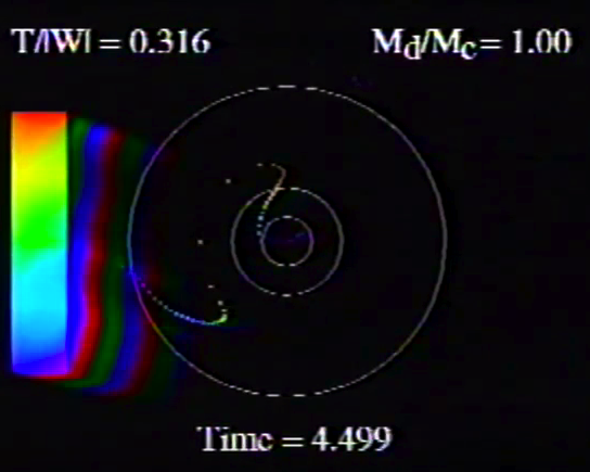
The middle panel of our Figure 2 is a reproduction of Figure 10 from WTH94. It shows the constant phase locus that emerged from the noise at late times during the evolution of four models: (a) Model O15; (b) model O14; (c) model E17; and (d) model E29. In the early '90s when this set of model simulations was carried out, we saved numerical data that detailed the time-evolutionary behavior of both the radial and azimuthal structure of each model's fastest growing eigenfunction. This data allowed us to generate after-the-fact, for example, plots of the constant phase locus at many different points in time to explicitly show how the azimuthally dependent eigenfunction developed out of the initial noise. Using techniques described in Tohline (2007), we transferred these plots, frame by frame, to VHS video tape so that this development could be viewed as an animation. Recently we have employed an analog-to-digital converter to create digital animations from nine of these analog VHS recordings, and each of the animations has been uploaded to YouTube. (The result of these analog-to-digital conversions was, unfortunately, digital animations of low fidelity. They are nevertheless informative.) Our Figure 2 displays a still image from, and provides a link to the YouTube animations that depict the time-evolutionary behavior of models O15 (upper left), O14 (upper right), E17 (lower left), and E29 (lower right); in order to play the desired YouTube video, click on the security-lock icon or the model name that accompanies the associated still image.
Links to five additional animation sequences are provided, immediately below, in our Figure 3. As is identified by the short caption accompanying each still image, these animations are from, respectively, models O13, O16, O17, O18, and O22.
| Figure 3: Five Additional Animation Sequences to Supplement Table 5 of WTH94 (click on security-lock icon or caption model name to go to YouTube) | ||||
|---|---|---|---|---|
| Table 5, Model O13 | Table 5, Model O16 | Table 5, Model O17 | Table 5, Model O18 | Table 5, Model O22 |
See Also
- Characteristics of Unstable Eigenvectors in Self-Gravitating Tori
- W. K. M. Rice, G. Lodato, & P. J. Armitage (2005), MNRAS, 364, L56-60. Investigating fragmentation conditions in self-gravitating accretion discs
This article describes 3D SPH simulations with 250,000 SPH particles in the disk and a single particle representing the central star. They address disk fragmentation in the context of rapid cooling of the disk. - J. E. Tohline (2007), Computing in Science & Engineering, vol. 9, no. 6, pp. 76 - 81. Scientific Visualization: A Necessary Chore … (PDF)

|
|---|
|
© 2014 - 2021 by Joel E. Tohline |

