Difference between revisions of "User:Tohline/SSC/Stability/BiPolytrope0 0CompareApproaches"
(→Sequences: Finished inserting and describing Figure 2) |
|||
| Line 178: | Line 178: | ||
<td align="left"> | <td align="left"> | ||
<math>~1 + 2\biggl(\frac{\rho_e}{\rho_c}\biggr) - 3\biggl(\frac{\rho_e}{\rho_c}\biggr)^2 | <math>~1 + 2\biggl(\frac{\rho_e}{\rho_c}\biggr) - 3\biggl(\frac{\rho_e}{\rho_c}\biggr)^2 | ||
\, | \, . | ||
</math> | </math> | ||
</td> | </td> | ||
| Line 184: | Line 184: | ||
</table> | </table> | ||
</div> | </div> | ||
This is equivalent to demanding that, | |||
<div align="center"> | <div align="center"> | ||
<table border="0" cellpadding="5" align="center"> | <table border="0" cellpadding="5" align="center"> | ||
| Line 196: | Line 196: | ||
</td> | </td> | ||
<td align="left"> | <td align="left"> | ||
<math>~\tfrac{1}{3}(1+2q^3) \, | <math>~\tfrac{1}{3}(1+2q^3) \, ,</math> | ||
</td> | </td> | ||
</tr> | </tr> | ||
</table> | </table> | ||
</div> | </div> | ||
and, simultaneously, | |||
<div align="center"> | |||
<table border="0" cellpadding="5" align="center"> | |||
<tr> | |||
<td align="right"> | |||
<math>~\frac{\rho_e}{\rho_c}</math> | |||
</td> | |||
<td align="center"> | |||
<math>~=</math> | |||
</td> | |||
<td align="left"> | |||
<math>~\tfrac{2q^3}{3}(1+2q^3) \, .</math> | |||
</td> | |||
</tr> | |||
</table> | |||
</div> | |||
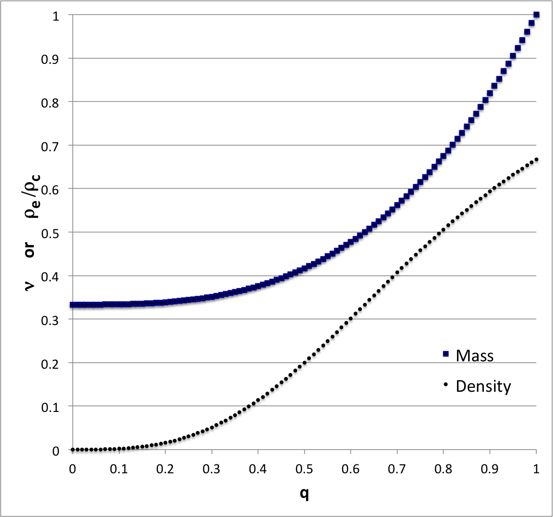
The behavior of these two functions is displayed in Figure 2; the variation of <math>~\nu</math> with <math>~q</math> is traced by the dark blue squares while the variation of <math>~\rho_e/\rho_c</math> with <math>~q</math> is marked by the small, circular black dots. | |||
=Related Discussions= | =Related Discussions= | ||
Revision as of 00:04, 7 January 2017
Comparing Stability Analyses of Zero-Zero Bipolytropes

|
|---|
| | Tiled Menu | Tables of Content | Banner Video | Tohline Home Page | |
In separate chapters we have discussed the following interrelated aspects of Bipolytropes that have <math>~(n_c,n_e) = (0,0)</math>:
- Using a detailed force-balance analysis to develop an analytic description of their equilibrium structure
- Using a free-energy analysis to analytically identify the properties of equilibrium structures; see also, an explicit, analytic evaluation of the statement of Virial Equilibrium
- Developing the Linear Adiabatic Wave Equation (LAWE) as it applies separately to the core and to the envelope of zero-zero bipolytropic configurations
- Identifying a method to analytically solve the matching LAWEs for a certain subset of configurations
- A summary of this solution technique, along with the first illustrative analytic specification of an eigenvector
- The derivation of analytically specifiable eigenvectors having a variety of mode quantum numbers
- A free-energy analysis of the global stability of zero-zero bipolytropes
Building on these separate discussions, here we examine what might be learned from a comparison of the two traditional approaches to stability analysis, namely: (1) solutions of the LAWE, and (2) a free-energy analysis.
Key Attributes of Equilibrium Configurations
Physical Properties
Aside from specifying its radius, <math>~R</math>, and total mass, <math>~M_\mathrm{tot}</math>, there are three particularly interesting dimensionless parameters that characterize the internal structure of a bipolytrope having <math>~(n_c,n_e) = (0,0)</math>. They are, the radial location of the core/envelope interface,
<math>~q \equiv \frac{r_i}{R} \, ;</math>
the ratio of the density of the envelope material to the density of the core, <math>~0 \le \rho_e/\rho_c \le 1</math>; and the fraction of the total mass that is contained in the core,
<math>~\nu \equiv \frac{M_\mathrm{core}}{M_\mathrm{tot}} \, .</math>
Identifying a unique bipolytropic configuration requires the specification of two of these three dimensionless parameters; the third parameter is, then, necessarily determined via the algebraic relation,
|
<math>~\frac{\rho_e}{\rho_c} </math> |
<math>=</math> |
<math>~\frac{q^3(1-\nu)}{\nu(1-q^3)} \, .</math> |
It is also relatively straightforward to appreciate that, in dimensional units, the value of the central density is,
|
<math>~\rho_c</math> |
<math>~=</math> |
<math>~\frac{3M_\mathrm{tot}}{4\pi G R^3} \cdot \frac{\nu}{q^3} \, .</math> |
Our study of equilibrium configurations has shown that once, for example, the pair of parameters, <math>~q</math> and <math>~\rho_e/\rho_c</math>, has been specified, other properties of the associated equilibrium configuration can be succinctly expressed in terms of the function,
|
<math>~g^2</math> |
<math>~\equiv</math> |
<math> 1 + \biggl(\frac{\rho_e}{\rho_c}\biggr) \biggl[ 2 \biggl(1 - \frac{\rho_e}{\rho_c} \biggr) \biggl( 1-q \biggr) + \frac{\rho_e}{\rho_c} \biggl(\frac{1}{q^2} - 1\biggr) \biggr] \, . </math> |
For example, the central pressure is given by the expression,
|
<math>~P_c</math> |
<math>~=</math> |
<math>\biggl( \frac{3}{2^3\pi} \biggr) \frac{\nu^2 g^2}{q^4} \biggl[ \frac{GM_\mathrm{tot}^2}{R^4} \biggr] \, .</math> |
Sequences
|
Across the two-dimensional, <math>~(q,\nu)</math> parameter space that is defined by the full range of physically viable values of <math>~q</math> and <math>~\nu</math>, namely,
<math>~0 \le q \le 1 \, ,</math> and <math>~0 \le \nu \le 1 \, ,</math>
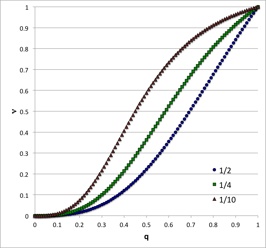
an equilibrium model sequence can be defined by, for example, specifying that all models along the sequence have the same density jump at the interface. Drawing on the above constraint relation, each choice of <math>~\rho_e/\rho_c</math> will generate a sequence governed by the function,
|
<math>~\nu</math> |
<math>=</math> |
<math>~\biggl[\frac{(1-q^3)}{q^3} \biggl( \frac{\rho_e}{\rho_c} \biggr) + 1\biggr]^{-1} </math> |
|
|
<math>=</math> |
<math>~\frac{q^3}{q^3 + (1-q^3)(\rho_e/\rho_c)} </math> |
Figure 1 displays several such equilibrium sequences across the <math>~(q,\nu)</math> plane — see also a related figure associated with our free-energy determination of stability. We have employed a free-energy analysis (see summary, below) to examine whether a transition from stable to unstable configurations is encountered while traversing — that is, while evolving along — such a sequence.
|
In a separate search for eigenvectors that simultaneously satisfy the linear adiabatic wave equation (LAWE) for the core and the LAWE for the envelope (see summary, below), we discovered that eigenvectors for some radial modes of oscillation can be specified fully analytically along a sequence of equilibrium models that is defined by the following constraint:
|
<math>~g^2</math> |
<math>~\equiv</math> |
<math>~1 + 2\biggl(\frac{\rho_e}{\rho_c}\biggr) - 3\biggl(\frac{\rho_e}{\rho_c}\biggr)^2 \, . </math> |
This is equivalent to demanding that,
|
<math>~\nu</math> |
<math>~=</math> |
<math>~\tfrac{1}{3}(1+2q^3) \, ,</math> |
and, simultaneously,
|
<math>~\frac{\rho_e}{\rho_c}</math> |
<math>~=</math> |
<math>~\tfrac{2q^3}{3}(1+2q^3) \, .</math> |
The behavior of these two functions is displayed in Figure 2; the variation of <math>~\nu</math> with <math>~q</math> is traced by the dark blue squares while the variation of <math>~\rho_e/\rho_c</math> with <math>~q</math> is marked by the small, circular black dots.
Related Discussions

|
|---|
|
© 2014 - 2021 by Joel E. Tohline |

