Excerpts from A Treatise of Fluxions

Both Volume I and Volume II of Colin Maclaurin's "A Treatise of Fluxions" can now be accessed online via Google Books. (Check out Wolfram's explanation of the term, fluxion.) In what follows, we provide an abbreviated table of contents for both volumes and present selected excerpts from these volumes.

Title Pages with Google-Books Links

Volume I (1^st Ed., 1742)	Volume II (2^nd Ed., 1801)

As is illustrated by the images displayed in the following two panels (click in one of the panels in order to view a higher-resolution image), each published "Figure Plate" was digitized (by Google Books) in segments that must be digitally pieced together in order to reconstruct some of the individual figures. See, for example, the discussion that references Fig. 282, below.

Example Digitized Figure Plates

Plate XXXII	Plate XXXIII

Volume I

Dedication (an 18^th Century Acknowledgment)
Preface
Introduction	1
Book 1 (Of the Fluxions of Geometrical Magnitudes)	51
Chapter I (Of the Grounds of this Method) — §§ 1-77	51
Chapter II (Of the Fluxions of plane rectilineal Figures) — §§ 78-104	109
Chapter III (Of the Fluxions of plane curvilineal Figures) — §§ 105-123	131
Chapter IV (Of the Fluxions of Solids, and of third Fluxions) — §§ 124-139	142
Chapter V (Of the Fluxions of Quantities that are in a continued Geometrical Progression, the first term of which is invariable) — §§ 140-150	152
Chapter VI (Of Logarithms, and of the Fluxions of logarithmic Quantities) — §§ 151-179	158
Chapter VII (Of the Tangents of curve Lines) — §§ 180-214	178
Chapter VIII (Of the Fluxions of curve Surfaces) — §§ 215-237	199
Chapter IX ([Identifying Extrema and Inflection Points] of Curves that are defined by a common or by a fluxional Equation) — §§ 238-285	214
Chapter X (Of the Asymptotes of curve Lines, the Areas bounded by them and …) — §§ 286-362	240
Chapter XI (Of the Curvature of Lines … different kinds of Contact [with other Curves] … Caustics … centripetal Forces …) — §§ 363-	304
· Parabola — §371	311
· Any Conic Section — §373	312
· The Second Fluxion of a Curve — §384	324
· Refraction of Light — §413	344
· Centripetal and Centrifugal Forces — §416	346
· Gravity — §419	348
· Circular Motion — §432	356
· When the Center of Forces is the Focus of a Conic Section — §446	370
· When Gravity is Uniform or Varies as any Power of the Distance — §458	383
· Orbit of the Moon, taking into account the Gravity of both the Earth and the Sun — §471	391
Extracted directly from §487 of Maclaurin's Book 1, as digitized by Google
· Prolate Spheroidal Fluid Figure — §491	409
Extracted directly from §491 of Maclaurin's Book 1, as digitized by Google
· The Earth's Equilibrium Shape — §492	410
Extracted directly from §492 of Maclaurin's Book 1, as digitized by Google
End of Book I, Chapter XI, § 494	413

Volume II

Table of Principal Contents (5 pp.)
Figure Plates (30 pp.)
Book 1 (continued)	1
Chapter XII (Of the Methods of Infinitesimals …) — §§ 495-570	1
· Centre of Gravity — §510	13
· Of the Collision of Bodies — §511	14
· Of the Descent of Bodies that Act upon One Another — §521	27
· Of the Centre of Oscillation — §533	40
· Of the Motion of Water Issuing from a Cylindric Vessel — §537	44
· Of the Catenaria — §551	59
· General Observations Concerning the Angles of Contact, etc. — §554	61
· General Observations Concerning centripetal Forces, etc. — §563	67
Chapter XIII (Determining the Lines of swiftest Descent in any Hypothesis of Gravity …) — §§ 571-608	74
· When Gravity is Directed Towards a Given Centre — §578	80
· Isoperimetrical Problems — §588	88
· The Solid of Least Resistance — §606	100
Chapter XIV (Of the Ellipse Considered as the Section of a Cylinder … Of the Figure of the Earth …) — §§ 609-	101
· Properties of the Ellipse — §609	101
· Of the Gravitation towards Spheres and Spheroids — §628	110
· Of the Figures of Planets (including effects of rotation) — §636	116
· Key Concluding Theorem! — §641	119
Extracted directly from §641 of Maclaurin's Book 1, as digitized by Google
· Using geometric relations, illustrate how to quantitatively determine gravitational acceleration …
[see related comment by Todhunter (1873), below]
▸ due to an arbitrarily shaped, uniform-density configuration — §642	120
▸ outside or on the surface of a uniform-density sphere — §643	121
▸ at the pole of an oblate spheroid — §644	122
▸ at the equator of an oblate spheroid — §645	123
▸ at both the pole and the equator of an oblong (i.e., prolate) spheroid — §647	125
▸ due to a pair of concentric, confocal spheroids — §648	127
· Apply Specifically to the Earth — §661	136
· What if the Earth's Density isn't Uniform but, instead, Varies Linearly with Distance? — §670	143
· Jupiter — §682	152
· Tides — §686	154
· Concluding Paragraph — §696	161
Extracted directly from §696 of Maclaurin's Book 1, as digitized by Google
End of Book I	162

Maclaurin's Discussion of Self-Gravitating, Oblate-Spheroidal Configurations

Paragraph (and related figure) extracted^† from Colin Maclaurin (1742) "A Treatise of Fluxions" Volume II, Chapter XIV, §628


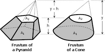
^†As displayed here (left panel), this paragraph has been pieced together from two text segments found on separate but sequential pages (pp. 110-111) of Google's digitized volume. The diagram labeled Fig. 283 (top-right panel) has been extracted from Maclaurin's Figure Plate XXXIII, which appears near the beginning of the same digitized file, and has been displayed here without modification. The diagrams in the bottom-right panel have been reposted from Mathalino.com in an effort to illustrate what Maclaurin means by "frustum of a cone."

Paragraph (and a pair of related diagrams) extracted^† from Colin Maclaurin (1742)

"A Treatise of Fluxions"

Volume II, Chapter XIV, §630

^†The paragraph (left panel) has been extracted from p. 111 of Google's digitized volume and displayed here without modification. The pair of diagrams (right panel) has been extracted from Figure Plate XXXIII, which appears near the beginning of the same digitized file. Note that the diagram on the right has been (poorly) pieced together from segments that appear on two separate pages of Google's digitized volume, presumably because the figure plate, itself, is folded in the original print publication.

Interpreting Maclaurin's Key Concluding Theorem

As noted above, in line with the table of contents for Volume II, the key theorem resulting from Maclaurin's analysis is …

Extracted directly from §641 of Maclaurin's Book 1, as digitized by Google

Here we assess this geometrically formulated statement using today's more common differential operators and algebraic expressions. In particular, we draw from the discussion of Maclaurin spheroids that has been presented in an accompanying chapter of this H_Book.

CA: This is the semi-minor (polar) axis of the spheroid, which we have called, <math>~a_3</math>.

CD: This is the semi-major (equatorial) radius of the spheroid, which we have called, <math>~a_1</math>.

With both <math>~a_1</math> and <math>~a_3</math> specified, the eccentricity of the oblate spheroid is also known via the expression,

<math>

e^2 \equiv 1 - \biggl(\frac{a_3}{a_1}\biggr)^2  .

</math>

Attraction of the Spheroid at the Pole: We interpret this phrase to mean the magnitude of the acceleration (force per unit mass) due to gravity at the pole, which is,

<math>~\mathcal{A} \equiv \biggl\|- \frac{\partial \Phi}{\partial z}\biggr\|_\mathrm{pole}</math>	<math>~=</math>	<math>~\pi G \rho \biggl\| \frac{\partial }{\partial z} \biggl[ I_\mathrm{BT} a_1^2 - \biggl(A_1 \varpi^2 + A_3 z^2 \biggr) \biggr]\biggr\|_\mathrm{pole} </math>
	<math>~=</math>	<math>~ 2\pi G \rho A_3 a_3 \, . </math>

Attraction at the Circumference of the Equator: We interpret this phrase to mean the magnitude of the acceleration (force per unit mass) due to gravity in the equatorial plane, at the surface of the configuration, which is,

<math>~\mathcal{D} \equiv \biggl\|- \frac{\partial \Phi}{\partial \varpi}\biggr\|_\mathrm{eq}</math>	<math>~=</math>	<math>~ \pi G \rho \biggl\| \frac{\partial }{\partial \varpi} \biggl[ I_\mathrm{BT} a_1^2 - \biggl(A_1 \varpi^2 + A_3 z^2 \biggr) \biggr]\biggr\|_\mathrm{eq} </math>
	<math>~=</math>	<math>~ 2\pi G \rho A_1 a_1 \, . </math>

Centrifugal force in the equatorial plane arising from rotation: We interpret this phrase to mean the centrifugal acceleration (force per unit mass) given by the expression,

<math>~\mathcal{V} \equiv \frac{(\varpi \omega_0)^2}{\varpi}\biggr|_\mathrm{eq}</math>

<math>~a_1\omega_0^2 \, .</math>

Maclaurin's theorem states that the rotating spheroidal configuration will be in equilibrium if,

<math>~\frac{\mathcal{D} - \mathcal{V}}{\mathcal{A}}</math>

or, equivalently,

<math>~\mathcal{D}-\mathcal{V}</math>

<math>~\mathcal{A}\biggl( \frac{a_3}{a_1} \biggr) \, .</math>

We choose to rewrite this expression and label it as,

Maclaurin's Theorem

<math>~\frac{\mathcal{V}}{a_1} = \frac{1}{a_1}\biggl[\mathcal{D} - \mathcal{A}\biggl( \frac{a_3}{a_1} \biggr)\biggr] </math>

which, in our terminology, becomes

<math>~\omega_0^2</math>	<math>~=</math>	<math>~2\pi G \rho \biggl[ A_1 - A_3\biggl( \frac{a_3}{a_1} \biggr)^2 \biggr] </math>
	<math>~=</math>	<math>~2\pi G \rho \biggl[A_1 - A_3(1-e^2) \biggr] \, .</math>

This is precisely the equilibrium frequency that we have derived elsewhere, from an evaluation of the gravitational potential of uniform-density spheroids.

Prolate Spheroid

As one specific example, Maclaurin discusses the gravitational attraction at the pole of a uniform-density, prolate spheroid in his §647 of Volume II (pp. 125-127). While his discussion of this topic necessarily refers back to earlier sections — most importantly, §643 (spheres) and §644 (oblate spheroids) — it frequently refers to Figure 291, No. 2, which we have reproduced in the following figure.

Figure extracted^† from Colin Maclaurin (1742)

"A Treatise of Fluxions"

Volume II, Figure Plate XXXIII

^†The .

In this animation sequence, the blue ellipse has an eccentricity, <math>~e = 0.55</math>, and the red line-segment is drawn at an angle to the horizontal axis that varies over the range, <math>~\tfrac{3\pi}{8} \ge \alpha \ge \tfrac{\pi}{8}</math>. As is described in the accompanying text, the orange curve — Maclaurin's "AKG" curve — is mapped out as the angle, <math>~\alpha</math>, is varied.

While trying to decipher Maclaurin's geometrically based derivation, we have found it useful to re-draw key elements of this figure, deriving relevant algebraic or trigonometric relations along the way. Because the "oblong" ellipse in Maclaurin's figure is oriented such that the axis of revolution — the symmetry axis — is horizontal, and because we prefer to associate the <math>~z</math> axis with the symmetry axis of the configuration, we will rather unconventionally refer to the horizontal axis as the <math>~z</math> (symmetry) axis. Adopting a cylindrical coordinate system furthermore means that, in our notation, the vertical axis will be the <math>~\varpi</math> axis.

The blue ellipse centered on the origin of our plot represents Maclaurin's "ADBE" ellipse; in the expressions that follow, we will use <math>~a_1</math> and <math>~a_3</math> to refer, respectively, to the length of the semi-major axis (Maclaurin's line-segment "CA") and semi-minor axis (Maclaurin's line-segment "CD") of the ellipse; and, following Maclaurin, we will refer to the leftmost point on the ellipse (Maclaurin's point "A") as the "pole" which is positioned at coordinate <math>~(z, \varpi) = (-a_1, 0)</math>. (Note that in our plot, we have set <math>~a_1 = 1</math>, but otherwise we will leave its specification arbitrary.) In our plot, Maclaurin's "CNH" circle is represented by the green quarter circle centered on the pole. The blue ellipse is defined by the relation,

<math>~\frac{z^2}{a_1^2} + \frac{\varpi^2}{a_3^2}</math>	<math>~=</math>	<math>~1 </math>
<math>~\Rightarrow ~~~~ \frac{z^2}{a_1^2} + (1-e^2)^{-1}\frac{\varpi^2}{a_1^2}</math>	<math>~=</math>	<math>~1 \, ,</math>

and, because it is off-center, the green quarter circle is defined by the relation,

<math>~(a_1 + z)^2 + \varpi^2</math>	<math>~=</math>	<math>~a_1^2 </math>
<math>~\Rightarrow ~~~~ \biggl(1 + \frac{z}{a_1} \biggr)^2 + \frac{\varpi^2}{a_1^2}</math>	<math>~=</math>	<math>~1 \, .</math>

The red line-segment in our plot is what Maclaurin refers to as "AM" which, in his words, is any right line from the pole A. We will use the variable, <math>~\alpha</math>, to identify the angle between this line-segment and the horizontal axis; in determining the gravitational attraction at pole A, Maclaurin ultimately sweeps this angle through the range, <math>~0 \le \alpha \le \tfrac{\pi}{2}</math>. Points lying along this line are defined by the relation,

<math>~\varpi</math>	<math>~=</math>	<math>~(a_1+z)\tan\alpha</math>
<math>~\Rightarrow ~~~~ \frac{\varpi}{a_1}</math>	<math>~=</math>	<math>~\biggl(1+\frac{z}{a_1}\biggr)\tan\alpha \, .</math>

Intersection With Circle

Hence, the red line-segment intersects the green quarter-circle when,

<math>~1- \biggl(1 + \frac{z}{a_1} \biggr)^2</math>	<math>~=</math>	<math>~\biggl(1+\frac{z}{a_1}\biggr)^2\tan^2\alpha </math>
<math>~\Rightarrow~~~~\biggl(1+\frac{z}{a_1}\biggr)^2(1+\tan^2\alpha)</math>	<math>~=</math>	<math>~1 </math>
<math>~\Rightarrow~~~~\frac{z}{a_1}</math>	<math>~=</math>	<math>~(1+\tan^2\alpha)^{-1/2} -1 </math>
	<math>~=</math>	<math>~\cos\alpha -1 \, .</math>

Correspondingly,

<math>\frac{\varpi}{a_1} = (\cos\alpha)\tan\alpha = \sin\alpha \, .</math>

Intersection With Ellipse

Similarly, the red line-segment intersects the blue ellipse when,

<math>~(1-e^2)\biggl[1- \biggl(\frac{z}{a_1} \biggr)^2\biggr]</math>	<math>~=</math>	<math>~\biggl(1+\frac{z}{a_1}\biggr)^2\tan^2\alpha </math>
<math>~\Rightarrow ~~~~ (1-e^2) - (1-e^2)\biggl(\frac{z}{a_1} \biggr)^2</math>	<math>~=</math>	<math>~\biggl[1+2\biggl(\frac{z}{a_1}\biggr)+\biggl(\frac{z}{a_1}\biggr)^2\biggr]\tan^2\alpha </math>
<math>~\Rightarrow ~~~~ 0</math>	<math>~=</math>	<math>~\biggl[\tan^2\alpha - (1-e^2)\biggr]+2\biggl(\frac{z}{a_1}\biggr)\tan^2\alpha +\biggl(\frac{z}{a_1}\biggr)^2\biggl[\tan^2\alpha+ (1-e^2) \biggr] \, .</math>

The roots of this quadratic equation are,

<math>~\frac{z}{a_1}</math>	<math>~=</math>	<math>~\frac{b}{2a}\biggl\{ -1 \pm \biggl[ 1 - \frac{4ac}{b^2} \biggr]^{1/2} \biggr\}</math>
	<math>~=</math>	<math>~\frac{\tan^2\alpha}{(\tan^2\alpha+ 1-e^2 )}\biggl\{ -1 \pm \biggl[ 1 - \frac{[\tan^2\alpha - (1-e^2)][ \tan^2\alpha+ (1-e^2) ]}{\tan^4\alpha} \biggr]^{1/2} \biggr\}</math>
	<math>~=</math>	<math>~\frac{\tan^2\alpha}{(\tan^2\alpha+ 1-e^2 )}\biggl\{ -1 \pm \frac{1}{\tan^2\alpha}\biggl[ \tan^4\alpha - [\tan^4\alpha - (1-e^2)^2] \biggr]^{1/2} \biggr\}</math>
	<math>~=</math>	<math>~-~\frac{[\tan^2\alpha \mp (1-e^2) ]}{[\tan^2\alpha+ (1-e^2 )]} \, .</math>

The "inferior" root gives,

<math>~\frac{z}{a_1}\biggr|_- = -1 \, ,</math>

while the "superior" root gives,

<math>~\frac{z}{a_1}\biggr|_+</math>

<math>~- ~\frac{[\tan^2\alpha - (1-e^2) ]}{[\tan^2\alpha+ (1-e^2) ]} \, .</math>

Correspondingly,

<math>\frac{\varpi}{a_1}\biggr|_- = 0 \, ,</math>

and,

<math>\frac{\varpi}{a_1}\biggr|_+ = \tan\alpha\biggl\{ 1 - ~\frac{[\tan^2\alpha - (1-e^2) ]}{[\tan^2\alpha+ (1-e^2) ]} \biggr\} \, .</math>

The "inferior" root clearly identifies the intersection of the red line-segment with the pole of the prolate spheroid. The "superior" root identifies the point at which the red line-segment intersects and crosses the blue ellipse, away from the pole.

Generate Curve AKG

In §644 (p. 122 of Volume II) of his Treatise, Maclaurin states that "the gravity at the pole A towards the spheroid ADBE will be measured by [the ratio],"

<math>\frac{\mathrm{AKGC}}{AC} \, ,</math>

where the numerator, "AKGC," is the area under the curve, "AKG," and the denominator is the length of the semi-major axis, <math>~a_1</math>. So a key element of Maclaurin's derivation is the proper construction of the curve, "AKG." The key sentence from his §644 appears to be the following:

Extracted directly from §644 of Maclaurin's Book 1, as digitized by Google

We interpret this phrase to mean that, as the angle, <math>~\alpha</math>, varies from <math>~\tfrac{\pi}{2}</math> to <math>~0</math>, the curve "AKG" is generated by plotting, as the ordinate, the length of the line-segment "AQ" and, as the abscissa, the <math>~z</math>-coordinate location of the vertical line, "RN" — we'll label this, <math>~z_\mathrm{RN}</math>. In our terminology, as derived above, <math>~z_\mathrm{RN}</math> is the <math>~z</math>-coordinate of the intersection of the red line-segment with the green quarter-circle, that is,

<math>~z_\mathrm{RN}</math>

<math>~\cos\alpha - 1 \, .</math>

And the magnitude of "AQ" is obtained from the <math>~z</math>-coordinate location of the vertical line, "MQ" — that is, the <math>~z</math>-coordinate of the intersection of the red line-segment with the blue ellipse — as derived above. Specifically, we interpret Maclaurin's phrase to mean that,

<math>~\frac{\mathrm{AQ}}{a_1} \equiv 1 + \frac{z}{a_1}\biggr|_+</math>

<math>~1 - ~\frac{[\tan^2\alpha - (1-e^2) ]}{[\tan^2\alpha+ (1-e^2) ]} \, .</math>

Using the first of these two expressions, we can rewrite the tangent function directly in terms of the ordinate, <math>~z_\mathrm{RN}</math>; specifically,

<math>\tan^2\alpha = \frac{1- \cos^2\alpha}{\cos^2\alpha} = \frac{1- (1+z_\mathrm{RN})^2}{(1+z_\mathrm{RN})^2} \, .</math>

Hence,

<math>~\frac{\mathrm{AQ}}{a_1} </math>	<math>~=</math>	<math>~1 - ~\frac{(1+z_\mathrm{RN})^2[\tan^2\alpha - (1-e^2) ]}{(1+z_\mathrm{RN})^2[\tan^2\alpha+ (1-e^2) ]}</math>
	<math>~=</math>	<math>~1 - ~\frac{[1-(1+z_\mathrm{RN})^2 - (1-e^2)(1+z_\mathrm{RN})^2 ]}{[1-(1+z_\mathrm{RN})^2+ (1-e^2) (1+z_\mathrm{RN})^2]}</math>
	<math>~=</math>	<math>~1 - ~\frac{[1+(1+z_\mathrm{RN})^2 (-1 - (1-e^2) ]}{[1+(1+z_\mathrm{RN})^2(-1+1-e^2)]}</math>
	<math>~=</math>	<math>~1 - ~\frac{[1-(2-e^2)(1+z_\mathrm{RN})^2 ]}{[1-e^2(1+z_\mathrm{RN})^2]}</math>
	<math>~=</math>	<math>~\frac{[1-e^2(1+z_\mathrm{RN})^2]-[1-(2-e^2)(1+z_\mathrm{RN})^2 ]}{[1-e^2(1+z_\mathrm{RN})^2]}</math>
	<math>~=</math>	<math>~\frac{[2(1-e^2)(1+z_\mathrm{RN})^2 ]}{[1-e^2(1+z_\mathrm{RN})^2]} \, .</math>

In our above figure, this function, <math>~\mathrm{AQ}(z_\mathrm{RN})</math> normalized to <math>~a_1</math>, is delineated by the orange triangles over the coordinate range, <math>~-1 \le z_\mathrm{RN} \le 0</math>. If our interpretation of Maclaurin's discussion is correct, this is precisely the curve in Maclauin's Figure 291, No. 2 that is labeled, "AKG."

Area Under the Curve

The area, "AKGC" — which, according to Maclaurin, gives the gravitational acceleration at the pole A — can be determined by carrying out the integral,

<math>~\frac{\mathrm{AKGC}}{a_1} </math>

<math>~\int_{-1}^0 \biggl[\frac{\mathrm{AQ}}{a_1}\biggr]dz_\mathrm{RN} \, .</math>

This integral can be more cleanly evaluated if we make the variable substitution,

<math>u_\mathrm{RN} \equiv 1 + z_\mathrm{RN} = \cos\alpha \, ,</math>

with a corresponding shift in the limits of integration from <math>~(-1 \rightarrow 0)</math>, for <math>~z_\mathrm{RN}</math>, to <math>~(0 \rightarrow 1)</math>, for <math>~u_\mathrm{RN}</math>. Specifically, we find,

<math>~\frac{\mathrm{AKGC}}{a_1} </math>	<math>~=</math>	<math>~2(1-e^2) \int_{0}^1 \frac{u_\mathrm{RN}^2 }{1-e^2 u_\mathrm{RN}^2} ~du_\mathrm{RN}</math>
	<math>~=</math>	<math>~-2(1-e^2) \biggl[ \frac{u_\mathrm{RN}}{e^2} \biggr]_{0}^1 + \frac{1}{e^4} \int_{0}^1 \frac{du_\mathrm{RN}}{e^{-2}- u_\mathrm{RN}^2} </math>
	<math>~=</math>	<math>~-\frac{2(1-e^2)}{e^2} + \frac{2(1-e^2)}{e^4} \biggl\{ \frac{e}{2} \ln \biggl[ \frac{e^{-2} +u_\mathrm{RN} }{e^{-2} -u_\mathrm{RN} } \biggr] \biggr\}_{0}^1 </math>
	<math>~=</math>	<math>~\frac{(1-e^2)}{e^3} \ln \biggl[ \frac{1 + e^{2} }{1-e^{2}} \biggr]-\frac{2(1-e^2)}{e^2} \, .</math>

This is precisely the expression for the coefficient, <math>~A_1</math>, that is traditionally used in the expression for the gravitational potential inside homogeneous, prolate spheroids.

Material that appears after this point in our presentation is under development and therefore
may contain incorrect mathematical equations and/or physical misinterpretations.
| Go Home |

Comparison With More Traditional Derivation

In our separate derivation of the gravitational acceleration at the pole of a prolate spheroid that uses a more traditional approach, we obtained this key coefficient by integrating over a different function, namely,

<math>~\mathcal{Z}</math>	<math>~\equiv</math>	<math>~\frac{(1-\zeta)}{ [ (2-e^2) - 2\zeta + e^2\zeta^2 ]^{1/2}} -1 </math>
	<math>~=</math>	<math>~\frac{(1-\zeta)^{1/2}}{ [ 2-e^2 - e^2\zeta ]^{1/2}} -1 \, .</math>

By comparing Maclaurin's approach to the more traditional one, we conclude that,

<math>~\int_{-1}^0 \biggl[\frac{\mathrm{AQ}}{a_1}\biggr]dz_\mathrm{RN} </math>

<math>~\int_{-1}^1 \mathcal{Z} d\zeta \, .</math>

We should be able to demonstrate explicitly that these two integrands are the same. We begin by recognizing that the relationship between the dimensionless coordinate, <math>~z/a_1</math>, that we have used to decipher Maclaurin's presentation and the dimensionless coordinate, <math>~\zeta</math>, that was used in our separate analysis, is,

Returning to the first expression in the above subsection that details the intersection of the red line-segment with the blue ellipse, we can therefore write,

<math>~(1-e^2) (1-\zeta^2)</math>	<math>~=</math>	<math>~(1-\zeta)^2\tan^2\alpha </math>
<math>~\Rightarrow~~~~ \tan^2\alpha </math>	<math>~=</math>	<math>~\frac{(1-e^2) (1+\zeta)}{(1-\zeta)} \, .</math>

Recalling that,

<math>u_\mathrm{RN} = \cos\alpha = [1+\tan^2\alpha]^{-1/2} \, ,</math>

we see that,

<math>~\frac{\mathrm{AQ}}{a_1} = \frac{2(1-e^2)u_\mathrm{RN}^2}{1-e^2 u_\mathrm{RN}^2}</math>	<math>~=</math>	<math>~\frac{2(1-e^2)[1+\tan^2\alpha]^{-1}}{1-e^2[1+\tan^2\alpha]^{-1}}</math>
	<math>~=</math>	<math>~\frac{2(1-e^2)}{1-e^2 +\tan^2\alpha}</math>
	<math>~=</math>	<math>~\frac{2(1-e^2)(1-\zeta)}{(1-e^2)(1-\zeta) +(1-e^2)(1+\zeta)}</math>
	<math>~=</math>	<math>~(1-\zeta) \, .</math>

Furthermore, we see that the transformation from <math>~u_\mathrm{RN}</math> to <math>~\zeta</math> is,

<math>~u_\mathrm{RN} = [1+\tan^2\alpha ]^{-1/2}</math>	<math>~=</math>	<math>~\biggl[1 + \frac{(1-e^2) (1+\zeta)}{(1-\zeta)} \biggr]^{-1/2}</math>
	<math>~=</math>	<math>~\biggl[\frac{(1-\zeta) + (1-e^2) (1+\zeta)}{(1-\zeta)} \biggr]^{-1/2}</math>
	<math>~=</math>	<math>~(1-\zeta)^{1/2} (2-e^2 -e^2\zeta)^{-1/2}</math>
<math>~\Rightarrow ~~~~ du_\mathrm{RN}</math>	<math>~=</math>	<math>~[ -2^{-1}(1-\zeta)^{-1/2} (2-e^2 -e^2\zeta)^{-1/2} -2^{-1}(1-\zeta)^{1/2} (2-e^2 -e^2\zeta)^{-3/2}(-e^2)]d\zeta </math>
	<math>~=</math>	<math>~-2^{-1}(1-\zeta)^{-1/2} (2-e^2 -e^2\zeta)^{-3/2}[ (2-e^2 -e^2\zeta)-e^2(1-\zeta) ]d\zeta </math>
	<math>~=</math>	<math>~-(1-e^2)(1-\zeta)^{-1/2} (2-e^2 -e^2\zeta)^{-3/2} d\zeta \, .</math>

Putting these two expressions together, we conclude that the integrand is,

<math>~\biggl[\frac{\mathrm{AQ}}{a_1}\biggr] du_\mathrm{RN}</math>	<math>~=</math>	<math>~-\biggl[\frac{(1-e^2)(1-\zeta)^{1/2} }{ (2-e^2 -e^2\zeta)^{3/2}}\biggr] d\zeta </math>
	<math>~=</math>	<math>~-\biggl[\frac{(1-e^2)}{(2-e^2 -e^2\zeta)} \biggr]\biggl[\frac{(1-\zeta)^{1/2} }{ (2-e^2 -e^2\zeta)^{1/2}}\biggr] d\zeta \, .</math>
	<math>~=</math>	<math>~-\biggl[\frac{(1-e^2)}{(2-e^2 -e^2\zeta)} \biggr]\biggl[1 + \mathcal{Z}\biggr] d\zeta \, .</math>

This does not appear to match the other integrand. I must be misinterpreting something!

To be done: I suspect that Maclaurin's approach will look more familiar if I redo the "traditional" derivation from the point of view of a spherical coordinate system (positioning pole A at the origin), in which an axisymmetric volume element takes the form,

<math>~dV = 2\pi r^2 \sin\alpha dr d\alpha = 2\pi r^2 dr du_\mathrm{RN} \, ,</math>

where, from above, <math>u_\mathrm{RN} \equiv \cos\alpha \, .</math>

Related Discussions

Our review of the Properties of Homogeneous Ellipsoids
Our derivation of the properties of Maclaurin Spheriods
Wikipedia's documentation of Colin Maclaurin
Chandrasekhar's (1967) historical account
Notes on the Life and Works of colin Maclaurin by Charles Tweedie (1919)
I. Todhunter (1873), A History of the Mathematical Theories of Attraction and the Figure of the Earth, from the time of Newton to that of Laplace. Note that Todhunter's discussion of Maclaurin's contributions can be found in Chapter IX, pp. 133-175.

Extracted directly from §252 of Todhunter's book, as digitized by xxx

User:Tohline/Apps/MaclaurinSpheroids/GoogleBooks

Contents