BiPolytrope with <math>n_c = 5</math> and <math>n_e=1</math>

Here we construct a bipolytrope in which the core has an <math>n_c=5</math> polytropic index and the envelope has an <math>n_c=1</math> polytropic index. This system is particularly interesting because the entire structure can be described by closed-form, analytic expressions. As far as I have been able to determine, this analytic structural model has not previously been published in a refereed, archival journal (author: Joel E. Tohline, March 30, 2013). In deriving the properties of this model, we will follow the general solution steps for constructing a bipolytrope that we have outlined elsewhere.

Steps 2 & 3

Based on the discussion presented elsewhere of the structure of an isolated <math>n=5</math> polytrope, the core of this bipolytrope will have the following properties:

<math> \theta(\xi) = \biggl[ 1 + \frac{1}{3}\xi^2 \biggr]^{-1/2} ~~~~\Rightarrow ~~~~ \theta_i = \biggl[ 1 + \frac{1}{3}\xi_i^2 \biggr]^{-1/2} ; </math>

<math> \frac{d\theta}{d\xi} = - \frac{\xi}{3}\biggl[ 1 + \frac{1}{3}\xi^2 \biggr]^{-3/2} ~~~~\Rightarrow ~~~~ \biggl(\frac{d\theta}{d\xi}\biggr)_i = - \frac{\xi_i}{3}\biggl[ 1 + \frac{1}{3}\xi_i^2 \biggr]^{-3/2} \, . </math>

The first zero of the function <math>\theta(\xi)</math> and, hence, the surface of the corresponding isolated <math>n=5</math> polytrope is located at <math>\xi_s = \infty</math>. Hence, the interface between the core and the envelope can be positioned anywhere within the range, <math>0 < \xi_i < \infty</math>.

Step 4: Throughout the core (<math>0 \le \xi \le \xi_i</math>)

Specify: <math>K_c</math> and <math>\rho_0 ~\Rightarrow</math>
<math>\rho</math>	<math>=</math>	<math>\rho_0 \theta^{n_c}</math>	<math>=</math>	<math>\rho_0 \biggl( 1 + \frac{1}{3}\xi^2 \biggr)^{-5/2}</math>
<math>P</math>	<math>=</math>	<math>K_c \rho_0^{1+1/n_c} \theta^{n_c + 1}</math>	<math>=</math>	<math>K_c \rho_0^{6/5} \biggl( 1 + \frac{1}{3}\xi^2 \biggr)^{-3}</math>
<math>r</math>	<math>=</math>	<math>\biggl[ \frac{(n_c + 1)K_c}{4\pi G} \biggr]^{1/2} \rho_0^{(1-n_c)/(2n_c)} \xi</math>	<math>=</math>	<math>\biggl[ \frac{K_c}{G\rho_0^{4/5}} \biggr]^{1/2} \biggl(\frac{3}{2\pi}\biggr)^{1/2} \xi</math>
<math>M_r</math>	<math>=</math>	<math>4\pi \biggl[ \frac{(n_c + 1)K_c}{4\pi G} \biggr]^{3/2} \rho_0^{(3-n_c)/(2n_c)} \biggl(-\xi^2 \frac{d\theta}{d\xi} \biggr)</math>	<math>=</math>	<math>\biggl[ \frac{K_c^3}{G^3 \rho_0^{2/5} } \biggr]^{1/2} \biggl( \frac{2\cdot 3}{\pi } \biggr)^{1/2} \biggl[ \xi^3 \biggl( 1 + \frac{1}{3}\xi^2 \biggr)^{-3/2} \biggr]</math>

Step 5: Interface Conditions

			Setting <math>n_c=5</math>, <math>n_e=1</math>, and <math>\phi_i = 1 ~~~~\Rightarrow</math>
<math>\frac{\rho_e}{\rho_0}</math>	<math>=</math>	<math>\biggl( \frac{\mu_e}{\mu_c} \biggr) \theta^{n_c}_i \phi_i^{-n_e}</math>	<math>=</math>	<math>\biggl( \frac{\mu_e}{\mu_c} \biggr) \theta^{5}_i </math>
<math>\biggl( \frac{K_e}{K_c} \biggr) </math>	<math>=</math>	<math>\rho_0^{1/n_c - 1/n_e}\biggl( \frac{\mu_e}{\mu_c} \biggr)^{-(1+1/n_e)} \theta^{1 - n_c/n_e}_i</math>	<math>=</math>	<math>\rho_0^{-4/5}\biggl( \frac{\mu_e}{\mu_c} \biggr)^{-2} \theta^{-4}_i</math>
<math>\frac{\eta_i}{\xi_i}</math>	<math>=</math>	<math>\biggl[ \frac{n_c + 1}{n_e+1} \biggr]^{1/2} \biggl( \frac{\mu_e}{\mu_c}\biggr) \theta_i^{(n_c-1)/2} \phi_i^{(1-n_e)/2}</math>	<math>=</math>	<math>3^{1/2} \biggl( \frac{\mu_e}{\mu_c}\biggr) \theta_i^{2}</math>
<math>\biggl( \frac{d\phi}{d\eta} \biggr)_i</math>	<math>=</math>	<math>\biggl[ \frac{n_c + 1}{n_e + 1} \biggr]^{1/2} \theta_i^{- (n_c + 1)/2} \phi_i^{(n_e+1)/2} \biggl( \frac{d\theta}{d\xi} \biggr)_i</math>	<math>=</math>	<math>3^{1/2} \theta_i^{- 3} \biggl( \frac{d\theta}{d\xi} \biggr)_i</math>

Step 6: Envelope Solution

Adopting equation (8) of Beech (1988), the most general solution to the <math>n=1</math> Lane-Emden equation can be written in the form,

<math> \phi = A \biggl[ \frac{\sin(\eta - B)}{\eta} \biggr] \, , </math>

where <math>A</math> and <math>B</math> are constants. The first derivative of this function is,

<math> \frac{d\phi}{d\eta} = \frac{A}{\eta^2} \biggl[ \eta\cos(\eta-B) - \sin(\eta-B) \biggr] \, . </math>

From Step 5, above, we know the value of the function, <math>\phi</math> and its first derivative at the interface; specifically,

<math> \phi_i = 1~~~~\mathrm{and} ~~~~\biggl( \frac{d\phi}{d\eta}\biggr)_i =3^{1/2} \theta_i^{- 3} \biggl( \frac{d\theta}{d\xi} \biggr)_i~~~~ \mathrm{at}~~~~\eta_i =3^{1/2} \xi_i \biggl( \frac{\mu_e}{\mu_c}\biggr) \theta_i^{2}</math>

From this information we can determine the constants <math>A</math> and <math>B</math>; specifically,

<math> \eta_i - B = \tan^{-1}(\Lambda_i^{-1}) = \frac{\pi}{2}- \tan^{-1}(\Lambda_i) \, , </math>

<math> A = \frac{\phi_i \eta_i}{\sin(\eta_i - B)} = \phi_i \eta_i (1 + \Lambda_i^2)^{1/2} \, , </math>

where,

<math> \Lambda_i = \frac{1}{\eta_i} + \frac{1}{\phi_i} \biggl(\frac{d\phi}{d\eta}\biggr)_i \, . </math>

Step 7

The surface will be defined by the location, <math>\eta_s</math>, at which the function <math>\phi(\eta)</math> first goes to zero, that is,

<math> \eta_s = \pi + B = \frac{\pi}{2} + \eta_i + \tan^{-1}(\Lambda_i) \, . </math>

Step 8: Throughout the envelope (<math>\eta_i \le \eta \le \eta_s</math>)

					Knowing: <math>K_e/K_c</math> and <math>\rho_e/\rho_0</math> from Step 5 <math>\Rightarrow</math>
<math>\rho</math>	<math>=</math>	<math>\rho_e \phi^{n_e}</math>	<math>=</math>	<math>\rho_0 \biggl(\frac{\rho_e}{\rho_0}\biggr) \phi</math>	<math>=</math>	<math>\rho_0 \biggl( \frac{\mu_e}{\mu_c} \biggr) \theta^{5}_i \phi</math>
<math>P</math>	<math>=</math>	<math>K_e \rho_e^{1+1/n_e} \phi^{n_e + 1}</math>	<math>=</math>	<math>K_c \rho_0^{6/5} \biggl(\frac{K_e \rho_0^{4/5}}{K_c}\biggr) \biggl(\frac{\rho_e}{\rho_0}\biggr)^{2} \phi^{2}</math>	<math>=</math>	<math>K_c \rho_0^{6/5} \theta^{6}_i \phi^{2}</math>
<math>r</math>	<math>=</math>	<math>\biggl[ \frac{(n_e + 1)K_e}{4\pi G} \biggr]^{1/2} \rho_e^{(1-n_e)/(2n_e)} \eta</math>	<math>=</math>	<math>\biggl[ \frac{K_c}{G \rho_0^{4/5}} \biggr]^{1/2} \biggl( \frac{K_e \rho_0^{4/5}}{K_c} \biggr)^{1/2} (2\pi)^{-1/2}\eta</math>	<math>=</math>	<math>\biggl[ \frac{K_c}{G \rho_0^{4/5}} \biggr]^{1/2} \biggl( \frac{\mu_e}{\mu_c} \biggr)^{-1} \theta^{-2}_i (2\pi)^{-1/2}\eta</math>
<math>M_r</math>	<math>=</math>	<math>4\pi \biggl[ \frac{(n_e + 1)K_e}{4\pi G} \biggr]^{3/2} \rho_e^{(3-n_e)/(2n_e)} \biggl(-\eta^2 \frac{d\phi}{d\eta} \biggr)</math>	<math>=</math>	<math>\biggl[ \frac{K_c^3}{G^3 \rho_0^{2/5}} \biggr]^{1/2} \biggl( \frac{K_e \rho_0^{4/5}}{K_c} \biggr)^{3/2} \biggl(\frac{\rho_e}{\rho_0}\biggr) \biggl( \frac{2}{\pi} \biggr)^{1/2} \biggl(-\eta^2 \frac{d\phi}{d\eta} \biggr)</math>	<math>=</math>	<math>\biggl[ \frac{K_c^3}{G^3 \rho_0^{2/5}} \biggr]^{1/2} \biggl( \frac{\mu_e}{\mu_c} \biggr)^{-2} \theta^{-1}_i \biggl( \frac{2}{\pi} \biggr)^{1/2} \biggl(-\eta^2 \frac{d\phi}{d\eta} \biggr)</math>

Examples

Normalization

The dimensionless variables used in Tables 1 & 2 are defined as follows:

<math>\rho^*</math>	<math>\equiv</math>	<math>\frac{\rho}{\rho_0}</math>	;	<math>r^*</math>	<math>\equiv</math>	<math>\frac{r}{[K_c^{1/2}/(G^{1/2}\rho_0^{2/5})]}</math>
<math>P^*</math>	<math>\equiv</math>	<math>\frac{P}{K_c\rho_0^{6/5}}</math>	;	<math>M_r^*</math>	<math>\equiv</math>	<math>\frac{M_r}{[K_c^{3/2}/(G^{3/2}\rho_0^{1/5})]}</math>
<math>H^*</math>	<math>\equiv</math>	<math>\frac{H}{K_c\rho_0^{1/5}}</math>	.

Parameter Values

The <math>2^\mathrm{nd}</math> column of Table 1 catalogues the analytic expressions that define various parameters and physical properties (as identified, respectively, in column 1) of the <math>n_c=5</math>, <math>n_e=1</math> bipolytrope. We have evaluated these expressions for various choices of the dimensionless interface radius, <math>\xi_i</math>, and have tabulated the results in the last few columns of the table. The tabulated values have been derived assuming <math>\mu_e/\mu_c = 1</math>, that is, assuming that the core and the envelope have the same mean molecular weights. The tabulated values of various parameters can be adjusted to correspond to other choices of this ratio by multiplying by the appropriate scaling coefficient as shown in column 1 of Table 1. For example, if the interface is positioned at <math>\xi_i = 0.5</math> but <math>\mu_e/\mu_c = 0.2</math>, then <math>\eta_i= 4.0</math> instead of <math>0.8</math>.

Table 1: Properties of <math>n_c=5</math>, <math>n_e=1</math>, BiPolytrope Having Various Interface Locations, <math>\xi_i</math>
File:BiPolytropeParametersV01.xml

Parameter	<math>\xi_i</math>	0.5	1.0	3.0
<math>\theta_i</math>	<math>\biggl( 1+\frac{1}{3}\xi_i^2 \biggr)^{-1/2}</math>	0.96077	0.86603	0.50000
<math>-\biggl(\frac{d\theta_i}{d\xi}\biggr)_i</math>	<math>\frac{1}{3} \xi_i \biggl( 1+\frac{1}{3}\xi_i^2 \biggr)^{-3/2}</math>	0.14781	0.21651	0.12500
<math>r^_\mathrm{core} \equiv r^_i</math>	<math>\biggl( \frac{3}{2\pi} \biggr)^{1/2} \xi_i</math>	0.34549	0.69099	2.07297
<math>\rho^_i \biggr\|_c = \biggl( \frac{\mu_e}{\mu_c} \biggr)^{-1} \rho^_i \biggr\|_e</math>	<math>\biggl( 1+\frac{1}{3}\xi_i^2 \biggr)^{-5/2}</math>	0.81864	0.48714	0.03125
<math>P^*_i</math>	<math>\biggl( 1+\frac{1}{3}\xi_i^2 \biggr)^{-3}</math>	0.78653	0.42188	0.01563
<math>H^_i \biggr\|_c = \frac{n_c+1}{n_e+1} \biggl( \frac{\mu_e}{\mu_c} \biggr) H^_i \biggr\|_e</math>	<math>6 \biggl( 1+\frac{1}{3}\xi_i^2 \biggr)^{-1/2}</math>	5.76461	5.19615	3.00000
<math>M^*_\mathrm{core}</math>	<math>\biggl( \frac{6}{\pi}\biggr)^{1/2} (\xi_i \theta_i)^3</math>	0.15320	0.89762	4.66417
<math>\biggl( \frac{\mu_e}{\mu_c} \biggr)^{-1}\eta_i</math>	<math>\sqrt{3} ~\theta_i^2 \xi_i</math>	0.79941	1.29904	1.29904
<math>-\biggl( \frac{d\phi}{d\eta} \biggr)_i</math>	<math>\sqrt{3} ~\theta_i^{-3} \biggl( - \frac{d\theta}{d\xi} \biggr)_i = \frac{\xi_i}{\sqrt{3}}</math>	0.28868	0.57735	1.73205
<math>\Lambda_i</math>	<math>\frac{1}{\eta_i} + \biggl( \frac{d\phi}{d\eta} \biggr)_i</math>	0.96225	0.19245	-0.96225
<math>A</math>	<math>\eta_i (1 + \Lambda_i^2)^{1/2}</math>	1.10940	1.32288	1.80278
<math>B</math>	<math>\eta_i - \frac{\pi}{2} + \tan^{-1}( \Lambda_i)</math>	- 0.00523	-0.08163	-1.03792
<math>\eta_s</math>	<math>\pi + B</math>	3.13637	3.05996	2.10367
<math>- \biggl( \frac{d\phi}{d\eta} \biggr)_s</math>	<math>\frac{A}{\eta_s}</math>	0.35372	0.43232	0.85697
<math>\biggl( \frac{\mu_e}{\mu_c} \biggr) \cdot \biggl[ R^* \equiv r^*_s \biggr]</math>	<math>\frac{\eta_s}{\sqrt{2\pi} ~\theta_i^2}</math>	1.35550	1.62766	3.35697
<math>\biggl( \frac{\mu_e}{\mu_c} \biggr)^2 M^*_\mathrm{tot}</math>	<math>\biggl(\frac{2}{\pi}\biggr)^{1/2} \theta_i^{-1} \biggl( -\eta^2 \frac{d\phi}{d\eta} \biggr)_s = \biggl(\frac{2}{\pi}\biggr)^{1/2} \frac{A\eta_s}{\theta_i}</math>	2.88959	3.72945	6.05187
<math>\biggl(\frac{\mu_e}{\mu_c}\biggr)^{-2} \cdot \biggl[ \nu \equiv \frac{M_\mathrm{core}}{M_\mathrm{tot}} \biggr]</math>	<math>\sqrt{3} ~\biggl( \frac{\xi_i^3 \theta_i^4}{A\eta_s} \biggr)</math>	0.05302	0.24068	0.77070
<math>\biggl(\frac{\mu_e}{\mu_c}\biggr)^{-1} \cdot \biggl[ q \equiv \frac{r_\mathrm{core}}{R} \biggr]</math>	<math>\sqrt{3}~\biggl[\frac{\xi_i \theta_i^2}{\eta_s}\biggr]</math>	0.25488	0.42453	0.61751

Profile

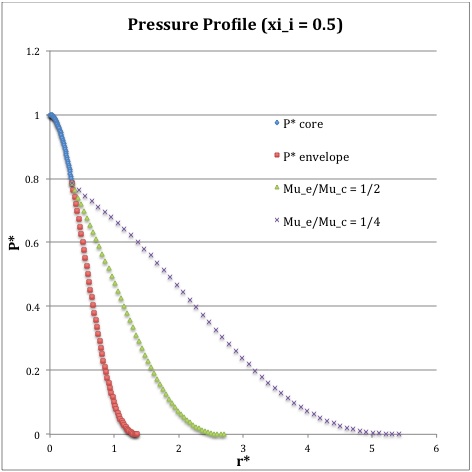
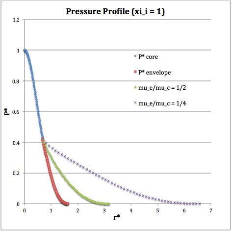
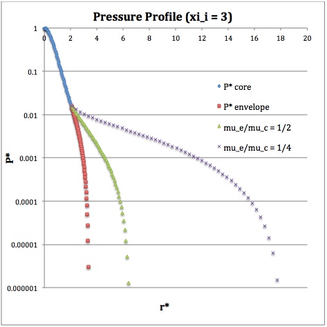
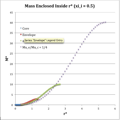
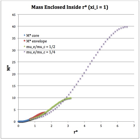
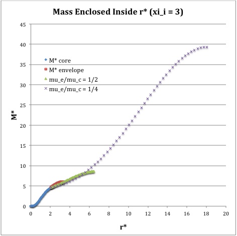
Once the values of the key set of parameters have been determined as illustrated in Table 1, the radial profile of various physical variables can be determined throughout the bipolytrope as detailed in step #4 and step #8, above. Table 2 summarizes the mathematical expressions that define the profile throughout the core (column 2) and throughout the envelope (column 3) of the normalized mass density, <math>\rho^*(r^*)</math>, the normalized gas pressure, <math>P^*(r^*)</math>, and the normalized mass interior to <math>r^*</math>, <math>M_r^*(r^*)</math>. For all profiles, the relevant normalized radial coordinate is <math>r^*</math>, as defined in the <math>2^\mathrm{nd}</math> row of Table 2. Graphical illustrations of these resulting profiles can be viewed by clicking on the thumbnail images posted in the last few columns of Table 2.

Table 2: Radial Profile of Various Physical Variables

Variable	Throughout the Core <math>0 \le \xi \le \xi_i</math>	Throughout the Envelope^† <math>\eta_i \le \eta \le \eta_s</math>	Plotted Profiles
Variable	Throughout the Core <math>0 \le \xi \le \xi_i</math>		<math>\xi_i = 0.5</math>	<math>\xi_i = 1.0</math>	<math>\xi_i = 3.0</math>
<math>r^*</math>	<math>\biggl( \frac{3}{2\pi} \biggr)^{1/2} \xi</math>	<math>\biggl( \frac{\mu_e}{\mu_c} \biggr)^{-1} \theta^{-2}_i (2\pi)^{-1/2}\eta</math>
<math>\rho^*</math>	<math>\biggl( 1 + \frac{1}{3}\xi^2 \biggr)^{-5/2}</math>	<math>\biggl( \frac{\mu_e}{\mu_c} \biggr) \theta^{5}_i \phi(\eta)</math>
<math>P^*</math>	<math>\biggl( 1 + \frac{1}{3}\xi^2 \biggr)^{-3}</math>	<math>\theta^{6}_i [\phi(\eta)]^{2}</math>
<math>M_r^*</math>	<math>\biggl( \frac{2\cdot 3}{\pi } \biggr)^{1/2} \biggl[ \xi^3 \biggl( 1 + \frac{1}{3}\xi^2 \biggr)^{-3/2} \biggr]</math>	<math>\biggl( \frac{\mu_e}{\mu_c} \biggr)^{-2} \theta^{-1}_i \biggl( \frac{2}{\pi} \biggr)^{1/2} \biggl(-\eta^2 \frac{d\phi}{d\eta} \biggr)</math>
^†In order to obtain the various envelope profiles, it is necessary to evaluate <math>\phi(\eta)</math> and its first derivative using the information presented in Step 6, above.

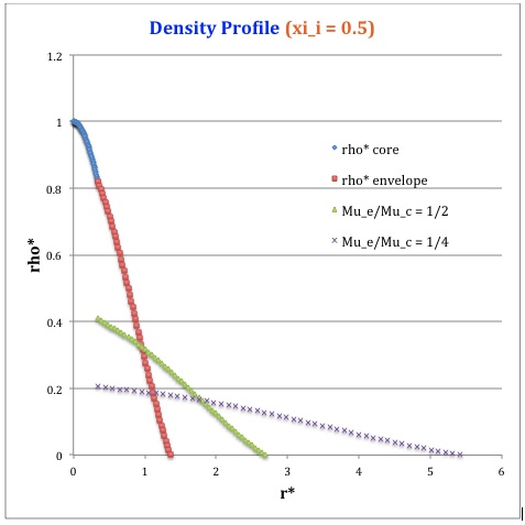
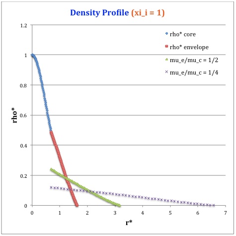
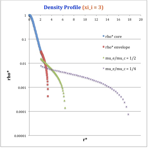
[As of 28 April 2013] For the interface locations <math>\xi_i = 0.5, ~1.0,~\mathrm{and}~3.0</math>, Table 2 provides profiles for three values of the molecular weight ratio: <math>\mu_e/\mu_c = 1.0, ~1/2,~\mathrm{and}~1/4</math>. In all nine graphs, blue diamonds trace the structure of the <math>n_c=5</math> core; the core extends to a radius, <math>r^*_\mathrm{core}</math>, that is independent of molecular weight ratio but varies in direct proportion to the choice of <math>\xi_i</math>. Specifically, as tabulated in the fourth row of Table 1, <math>r^*_\mathrm{core} = 0.34549, ~0.69099, ~\mathrm{and} ~2.07297</math> for, respectively, <math>\xi_i = 0.5,~1,~\mathrm{and}~3</math>. Notice that, while the pressure profile and mass profile are continuous at the interface for all choices of the molecular weight ratio, the density profile exhibits a discontinuous jump that is in direct proportion to the chosen value of <math>\mu_e/\mu_c</math>.

Throughout the envelope, the profile of all physical variables varies with the choice of the molecular weight ratio. In the Table 2 graphs, red squares trace the envelope profile for <math>\mu_e/\mu_c = 1.0</math>; green triangles trace the envelope profile for <math>\mu_e/\mu_c = 1/2</math>; and purple crosses trace the envelope profile for <math>\mu_e/\mu_c = 1/4</math>. The surface of the bipolytropic configuration is defined by the (normalized) radius, <math>R^*</math>, at which the envelope density and pressure drop to zero; the values tabulated in row 16 of Table 1 — <math>1.35550, ~1.62766, ~\mathrm{and} ~3.35697</math> for, respectively, <math>\xi_i = 0.5,~1,~\mathrm{and}~3</math> — correspond to a molecular weight ratio of unity and, hence also, to the envelope profiles traced by red squares in the Table 2 graphs. As the molecular weight ratio is decreased from unity to <math>1/2</math> and, then, <math>1/4</math> for a given choice of <math>\xi_i</math>, the (normalized) radius of the bipolytrope increases roughly in inverse proportion to <math>\mu_e/\mu_c</math> as suggested by the formula for <math>R^*</math> shown in Table 1. This proportional relation is not exact, however, because the parameter <math>\eta_s</math>, which also appears in the formula for <math>R^*</math>, contains an implicit dependence on the chosen value of the molecular weight ratio through the parameter <math>\eta_i</math>.

For a given choice of the interface parameter, <math>\xi_i</math>, the (normalized) mass that is contained in the core is independent of the choice of the molecular weight ratio. However, the (normalized) total mass, <math>M_\mathrm{tot}^*</math>, varies significantly with the choice of <math>\mu_e/\mu_c</math>; as suggested by the expression provided in row 17 of Table 1, the variation is in rough proportion to <math>(\mu_e/\mu_c)^{-2}</math> but, as with <math>R^*</math>, this proportional relation is not exact because the parameters <math>\eta_s</math> and <math>A</math> harbor an implicit dependence on the molecular weight ratio.

Model Sequences

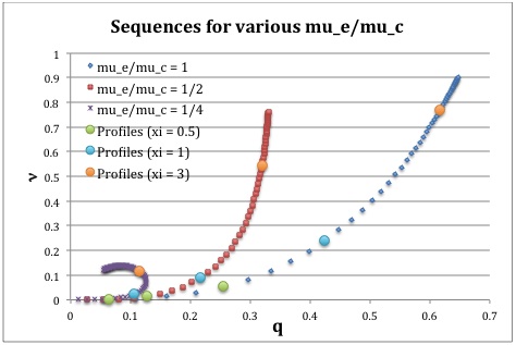
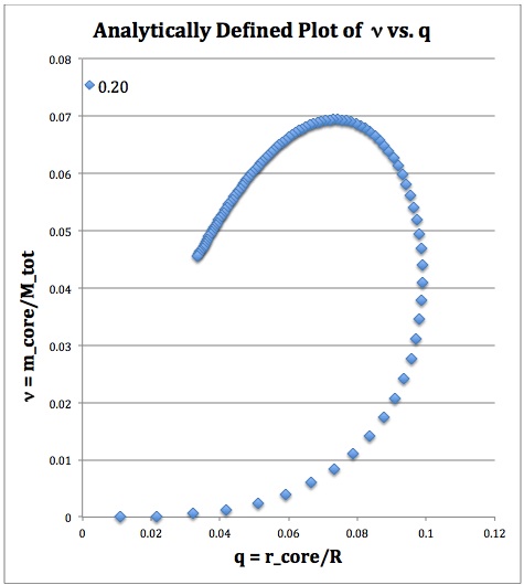
For a given choice of <math>\mu_e/\mu_c</math> a physically relevant sequence of models can be constructed by steadily increasing the value of <math>\xi_i</math> from zero to infinity — or at least to some value, <math>\xi_i \gg 1</math>. The blue curve shown on the left-hand side of Figure 1 presents one such model sequence, generated for the choice <math>\mu_e/\mu_c = 0.2</math>. The curve shows how the fractional core mass, <math>\nu \equiv M_\mathrm{core}/M_\mathrm{tot}</math>, varies in relation to the fractional core radius, <math>q \equiv r^*_\mathrm{core}/R^*_\mathrm{tot}</math>; the analytic expressions for these two ratios are presented in the last two rows of Table 1.

The expectation is that an increase in <math>\xi_i</math> along the sequence will correspond to an increase in the size — both the radius and the mass — of the core. This expectation is realized

Figure 1: Fractional mass versus fractional radius along the equilibrium sequence
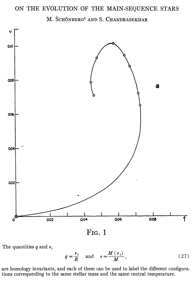
Analytic BiPolytrope with <math>n_c=5</math>, <math>n_e = 1</math>, and <math>\mu_e/\mu_c = 0.2</math>	Edited excerpt from Schönberg & Chandrasekhar (1942)

Plot of fractional core mass (<math>\nu</math>) versus fractional core radius (<math>q</math>) for the analytic bipolytrope having <math>\mu_e/\mu_c = 0.2</math>. The behavior of this analytically defined model sequence closely resembles the behavior of the numerically constructed isothermal core model presented by Schönberg & Chandrasekhar (1942).

Related Discussions

BiPolytropes Introduction

User:Tohline/SSC/Structure/BiPolytropes/Analytic5 1

Contents