Difference between revisions of "User:Tohline/SSC/Stability/BiPolytropes"
| Line 20: | Line 20: | ||
</tr> | </tr> | ||
</table> | </table> | ||
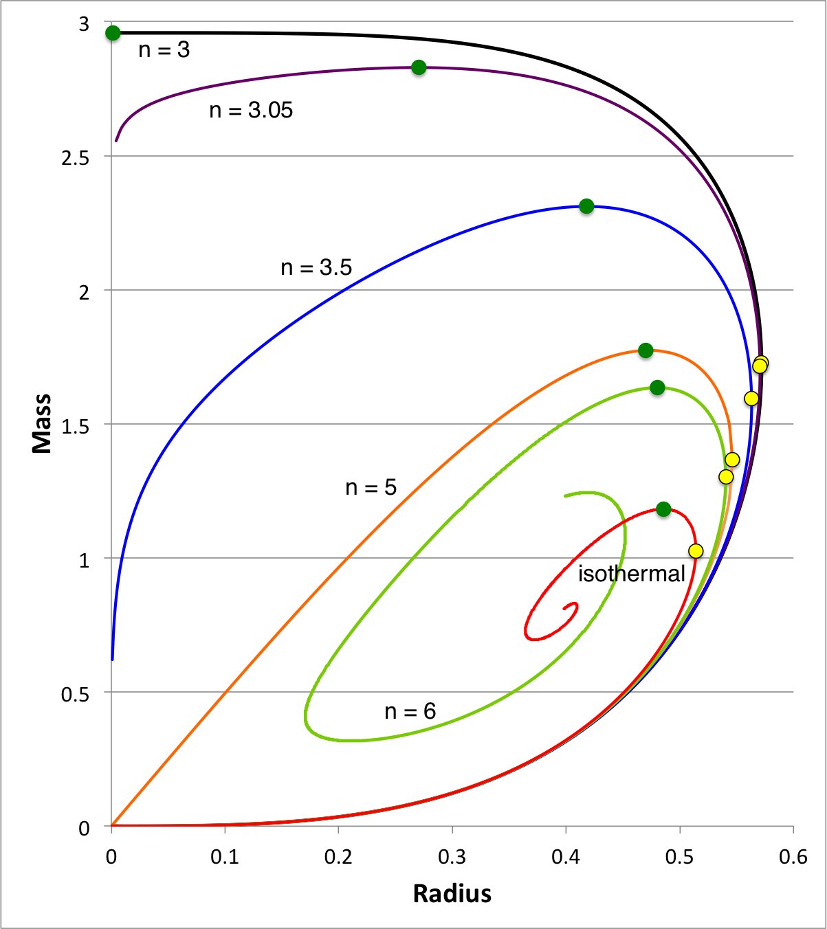
We expect the content of this chapter — which examines the relative stability of bipolytropes — to parallel in many ways the content of an [[User:Tohline/SSC/Stability/InstabilityOnsetOverview#Marginally_Unstable_Pressure-Truncated_Gas_Clouds|accompanying chapter in which we have successfully analyzed the relative stability of pressure-truncated polytopes]]. Figure 1, shown here on the right, has been copied from that separate discussion. The curves show the mass-radius relationship for pressure-truncated model sequences having a variety of polytropic indexes, as labeled, over the range <math>3 \le n \le \infty</math>. On each sequence, the green filled circle identifies the model with the largest mass. We have shown that the oscillation frequency of the fundamental-mode of radial oscillation is precisely zero for each one of these maximum-mass models. As a consequence, we know that each green circular marker identifies the point along its associated sequence that separates dynamically stable from dynamically unstable models. | We expect the content of this chapter — which examines the relative stability of bipolytropes — to parallel in many ways the content of an [[User:Tohline/SSC/Stability/InstabilityOnsetOverview#Marginally_Unstable_Pressure-Truncated_Gas_Clouds|accompanying chapter in which we have successfully analyzed the relative stability of pressure-truncated polytopes]]. Figure 1, shown here on the right, has been copied from that separate discussion. The curves show the mass-radius relationship for pressure-truncated model sequences having a variety of polytropic indexes, as labeled, over the range <math>3 \le n \le \infty</math>. On each sequence, the green filled circle identifies the model with the largest mass. We have shown ''analytically'' that the oscillation frequency of the fundamental-mode of radial oscillation is precisely zero<sup>†</sup> for each one of these maximum-mass models. As a consequence, we know that each green circular marker identifies the point along its associated sequence that separates dynamically stable (larger radii) from dynamically unstable (smaller radii) models. | ||
---- | |||
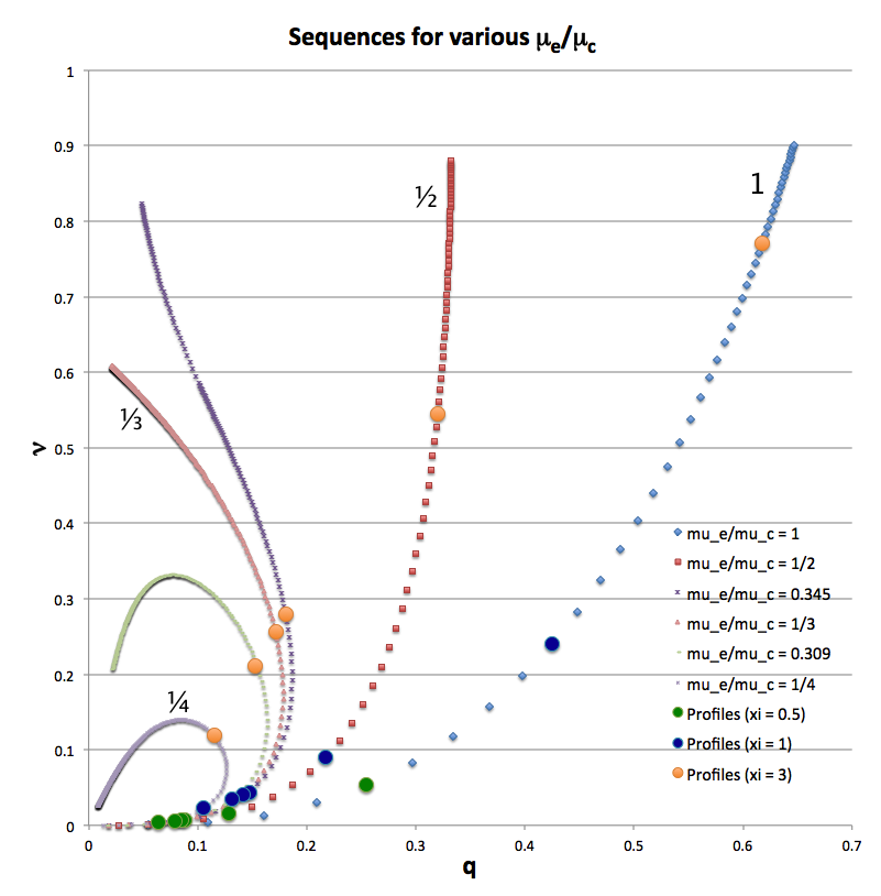
For a given choice of <math>~\mu_e/\mu_c</math> a physically relevant sequence of models can be constructed by steadily increasing the value of <math>\xi_i</math> from zero to infinity — or at least to some value, <math>\xi_i \gg 1</math>. Figure 2 shows how the fractional core mass, <math>\nu \equiv M_\mathrm{core}/M_\mathrm{tot}</math>, varies with the fractional core radius, <math>q \equiv r_\mathrm{core}/R</math>, along sequences having six different values of <math>~\mu_e/\mu_c</math>, as detailed in the figure caption. The natural expectation is that an increase in <math>\xi_i</math> along a given sequence will correspond to an increase in the relative size — both the radius and the mass — of the core. This expectation is realized along the sequences marked by blue diamonds (<math>~\mu_e/\mu_c = 1</math>) and by red squares (<math>~\mu_e/\mu_c = </math>½). But the behavior is different along the other four illustrated sequences. For sufficiently large <math>~\xi_i</math>, the relative radius of the core begins to decrease; then, as <math>~\xi_i</math> is pushed to even larger values, eventually the relative core mass begins to decrease. Additional properties of these equilibrium sequences are discussed in [[User:Tohline/SSC/FreeEnergy/PolytropesEmbedded#Behavior_of_Equilibrium_Sequence|an accompanying chapter]]. | <sup>†</sup>In each case, the fundamental-mode oscillation frequency is precisely zero if, and only if, the adiabatic index governing expansions/contractions is related to the underlying ''structural'' polytropic index via the relation, <math>~\gamma_g = (n + 1)/n</math>, and if a constant surface-pressure boundary condition is imposed. | ||
---- | |||
In yet another [[User:Tohline/SSC/Structure/BiPolytropes/Analytic5_1#BiPolytrope_with_nc_.3D_5_and_ne_.3D_1|accompanying chapter]], we have used purely analytic techniques to construct equilibrium sequences of spherically symmetric bipolytropes that have, <math>~(n_c,n_e) = (5,1)</math>. For a given choice of <math>~\mu_e/\mu_c</math> a physically relevant sequence of models can be constructed by steadily increasing the value of <math>\xi_i</math> from zero to infinity — or at least to some value, <math>\xi_i \gg 1</math>. Figure 2 shows how the fractional core mass, <math>\nu \equiv M_\mathrm{core}/M_\mathrm{tot}</math>, varies with the fractional core radius, <math>q \equiv r_\mathrm{core}/R</math>, along sequences having six different values of <math>~\mu_e/\mu_c</math>, as detailed in the figure caption. The natural expectation is that an increase in <math>\xi_i</math> along a given sequence will correspond to an increase in the relative size — both the radius and the mass — of the core. This expectation is realized along the sequences marked by blue diamonds (<math>~\mu_e/\mu_c = 1</math>) and by red squares (<math>~\mu_e/\mu_c = </math>½). But the behavior is different along the other four illustrated sequences. For sufficiently large <math>~\xi_i</math>, the relative radius of the core begins to decrease; then, as <math>~\xi_i</math> is pushed to even larger values, eventually the relative core mass begins to decrease. Additional properties of these equilibrium sequences are discussed in [[User:Tohline/SSC/FreeEnergy/PolytropesEmbedded#Behavior_of_Equilibrium_Sequence|an accompanying chapter]]. | |||
<div align="center"> | <div align="center"> | ||
<table border="0" cellpadding="5" width="30%"> | <table border="0" cellpadding="5" width="30%"> | ||
<tr> | <tr> | ||
<th colspan="2" align="center">Figure 2:</th> | <th colspan="2" align="center">Figure 2: Equilibrium Sequences of Bipolytropes with <math>~(n_c,n_e) = (5,1)</math></th> | ||
</tr> | </tr> | ||
<tr> | <tr> | ||
Revision as of 16:02, 2 November 2018
Marginally Unstable Bipolytropes
Our aim is to determine whether or not there is a relationship between equilibrium models at turning points along bipolytrope sequences and bipolytropic models that are marginally (dynamically) unstable toward collapse (or dynamical expansion).

|
|---|
| | Tiled Menu | Tables of Content | Banner Video | Tohline Home Page | |
| Figure 1: Equilibrium Sequences of Pressure-Truncated Polytropes |
|---|
We expect the content of this chapter — which examines the relative stability of bipolytropes — to parallel in many ways the content of an accompanying chapter in which we have successfully analyzed the relative stability of pressure-truncated polytopes. Figure 1, shown here on the right, has been copied from that separate discussion. The curves show the mass-radius relationship for pressure-truncated model sequences having a variety of polytropic indexes, as labeled, over the range <math>3 \le n \le \infty</math>. On each sequence, the green filled circle identifies the model with the largest mass. We have shown analytically that the oscillation frequency of the fundamental-mode of radial oscillation is precisely zero† for each one of these maximum-mass models. As a consequence, we know that each green circular marker identifies the point along its associated sequence that separates dynamically stable (larger radii) from dynamically unstable (smaller radii) models.
†In each case, the fundamental-mode oscillation frequency is precisely zero if, and only if, the adiabatic index governing expansions/contractions is related to the underlying structural polytropic index via the relation, <math>~\gamma_g = (n + 1)/n</math>, and if a constant surface-pressure boundary condition is imposed.
In yet another accompanying chapter, we have used purely analytic techniques to construct equilibrium sequences of spherically symmetric bipolytropes that have, <math>~(n_c,n_e) = (5,1)</math>. For a given choice of <math>~\mu_e/\mu_c</math> a physically relevant sequence of models can be constructed by steadily increasing the value of <math>\xi_i</math> from zero to infinity — or at least to some value, <math>\xi_i \gg 1</math>. Figure 2 shows how the fractional core mass, <math>\nu \equiv M_\mathrm{core}/M_\mathrm{tot}</math>, varies with the fractional core radius, <math>q \equiv r_\mathrm{core}/R</math>, along sequences having six different values of <math>~\mu_e/\mu_c</math>, as detailed in the figure caption. The natural expectation is that an increase in <math>\xi_i</math> along a given sequence will correspond to an increase in the relative size — both the radius and the mass — of the core. This expectation is realized along the sequences marked by blue diamonds (<math>~\mu_e/\mu_c = 1</math>) and by red squares (<math>~\mu_e/\mu_c = </math>½). But the behavior is different along the other four illustrated sequences. For sufficiently large <math>~\xi_i</math>, the relative radius of the core begins to decrease; then, as <math>~\xi_i</math> is pushed to even larger values, eventually the relative core mass begins to decrease. Additional properties of these equilibrium sequences are discussed in an accompanying chapter.
| Figure 2: Equilibrium Sequences of Bipolytropes with <math>~(n_c,n_e) = (5,1)</math> | |
|---|---|
|
Figure 2: Analytically determined plot of fractional core mass (<math>~\nu</math>) versus fractional core radius (<math>~q</math>) for <math>~(n_c, n_e) = (5, 1)</math> bipolytrope model sequences having six different values of <math>~\mu_e/\mu_c</math>: 1 (blue diamonds), ½ (red squares), 0.345 (dark purple crosses), ⅓ (pink triangles), 0.309 (light green dashes), and ¼ (purple asterisks). Along each of the model sequences, points marked by solid-colored circles correspond to models whose interface parameter, <math>~\xi_i</math>, has one of three values: 0.5 (green circles), 1 (dark blue circles), or 3 (orange circles); the images linked to Table 2 provide plots of the density, pressure and mass profiles for nine of these identified models. |
See Also

|
|---|
|
© 2014 - 2021 by Joel E. Tohline |

