Difference between revisions of "User:Tohline/Appendix/Ramblings/ForOuShangli"
(Created page with '<!-- __FORCETOC__ will force the creation of a Table of Contents --> <!-- __NOTOC__ will force TOC off --> =For Shangli Ou= {{LSU_HBook_header}} ==Context== <span id="Fig2">&n…') |
|||
| Line 5: | Line 5: | ||
{{LSU_HBook_header}} | {{LSU_HBook_header}} | ||
== | ==EFE Diagram== | ||
<span id=" | <span id="Fig1"> </span> | ||
<table border=" | <table border="0" cellpadding="5" width="90%" align="center"> | ||
<tr><td align=" | <tr> | ||
<td align="left" rowspan=" | <td align="left"> | ||
[[File:EFEdiagram4.png|left|500px|EFE Diagram identifying example models from Ou (2006)]] | |||
</td> | |||
<td align="left" rowspan="1"> | |||
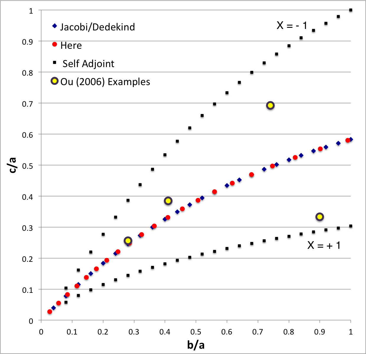
In the context of our broad discussion of ellipsoidal figures of equilibrium, the label "EFE Diagram" refers to a two-dimensional parameter space defined by the pair of axis ratios (b/a, c/a), ''usually'' covering the ranges, 0 ≤ b/a ≤ 1 and 0 ≤ c/a ≤ 1. The classic/original version of this diagram appears as Figure 2 on p. 902 of [http://adsabs.harvard.edu/abs/1965ApJ...142..890C S. Chandrasekhar (1965, ApJ, vol. 142, pp. 890-921)]; a somewhat less cluttered version appears on p. 147 of Chandrasekhar's [<b>[[User:Tohline/Appendix/References#EFE|<font color="red">EFE</font>]]</b>]. | In the context of our broad discussion of ellipsoidal figures of equilibrium, the label "EFE Diagram" refers to a two-dimensional parameter space defined by the pair of axis ratios (b/a, c/a), ''usually'' covering the ranges, 0 ≤ b/a ≤ 1 and 0 ≤ c/a ≤ 1. The classic/original version of this diagram appears as Figure 2 on p. 902 of [http://adsabs.harvard.edu/abs/1965ApJ...142..890C S. Chandrasekhar (1965, ApJ, vol. 142, pp. 890-921)]; a somewhat less cluttered version appears on p. 147 of Chandrasekhar's [<b>[[User:Tohline/Appendix/References#EFE|<font color="red">EFE</font>]]</b>]. | ||
| Line 24: | Line 27: | ||
</td> | </td> | ||
</tr> | </tr> | ||
</table> | |||
==Example 3D Interactive Animations== | |||
===b41c385=== | |||
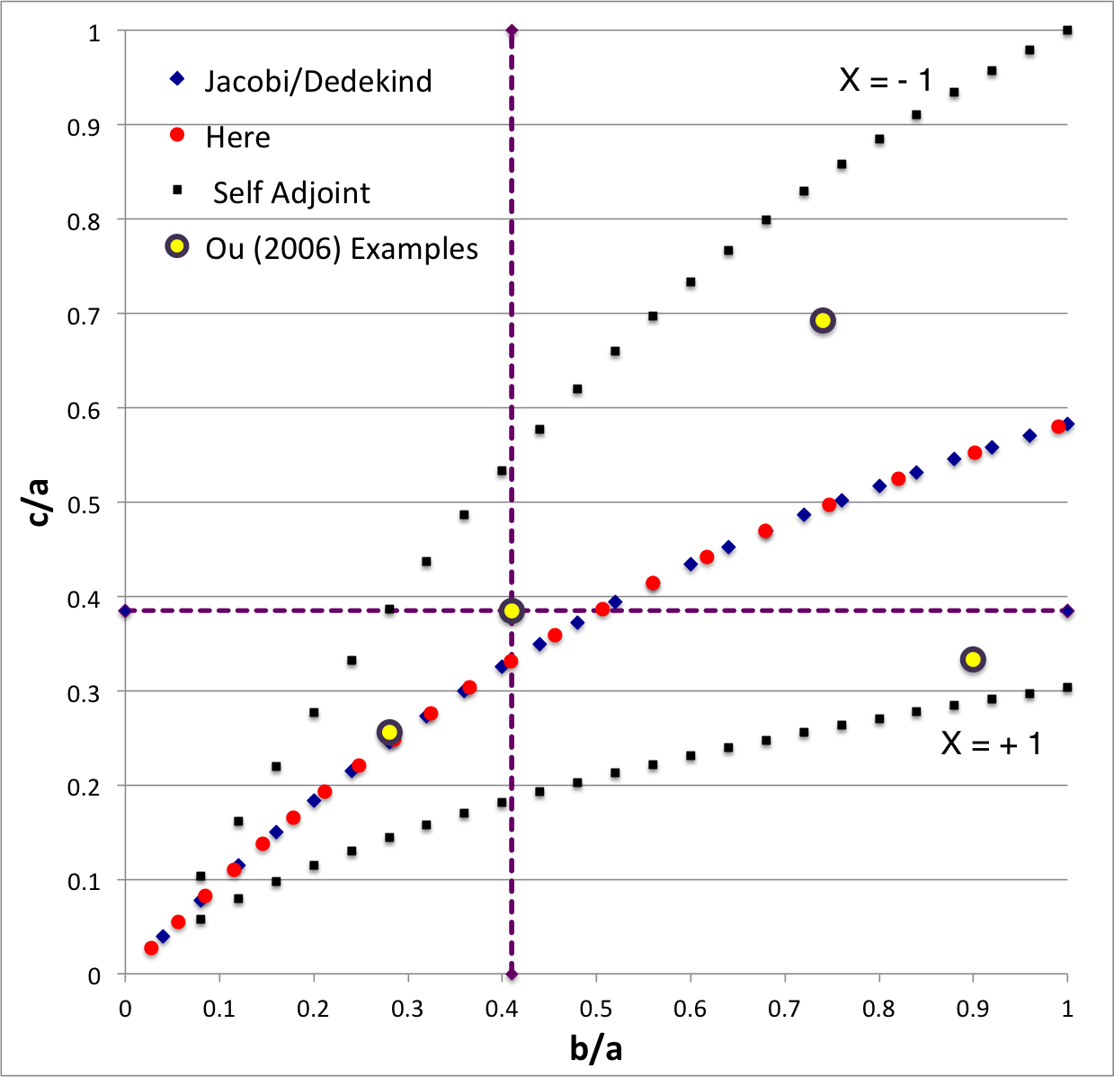
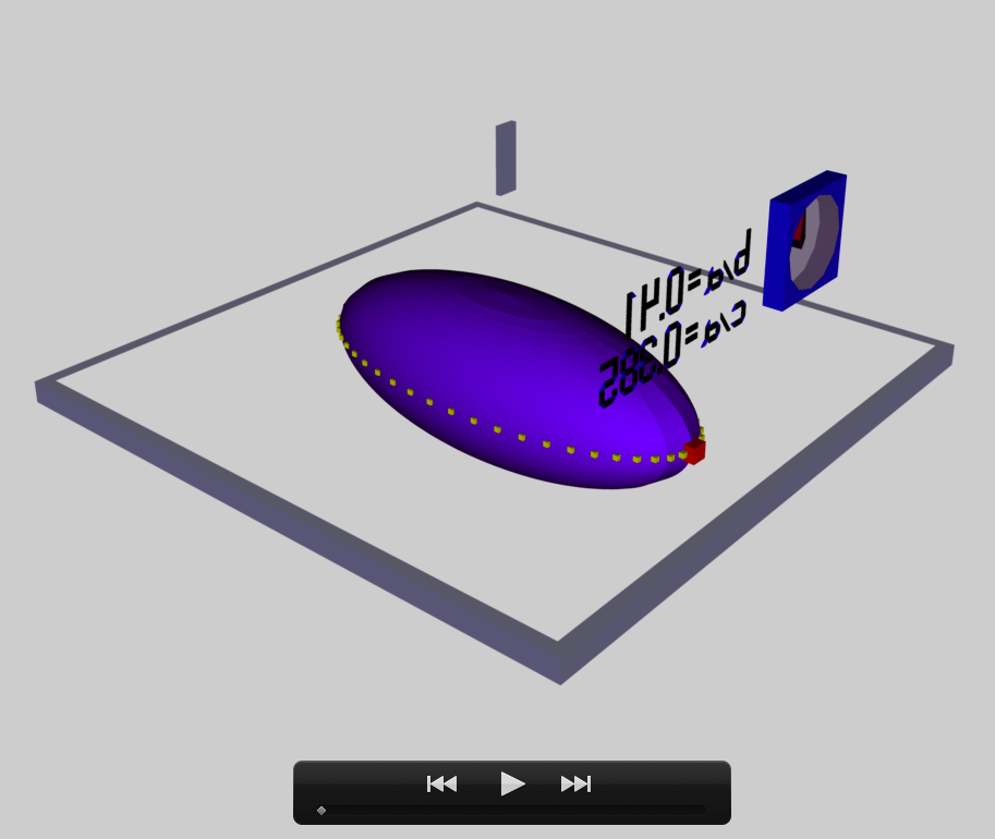
The model that we have chosen to use in our first successful construction of a COLLADA-based, 3D and interactive animation has the following properties; this model has been selected from [[User:Tohline/ThreeDimensionalConfigurations/RiemannStype#Table2|Table 2 of our accompanying discussion of Riemann S-type ellipsoids]]: | |||
<table border="0" cellpadding="5" align="center"> | |||
<tr> | |||
<td align="center" rowspan="6"> | |||
<b>Figure 1a</b><br /> <br /> | |||
[[File:B41c385EFEdiagram02.png|325px|EFE Parameter Space]] | |||
</td> | |||
<td align="center" rowspan="6" width="2%"> | |||
| |||
</td> | |||
<td align="center" colspan="3"> | |||
<math>~\frac{b}{a} = 0.41</math> | |||
</td> | |||
<td align="center" rowspan="6" width="2%"> | |||
| |||
</td> | |||
<td align="center" rowspan="6" bgcolor="lightgrey"> | |||
<b>Figure 1b</b><br /> | |||
[[File:COLLADA3rdViewpoint.png|300px|EFE Model b41c385]] | |||
</td> | |||
</tr> | |||
<tr> | |||
<td align="center" colspan="3"> | |||
<math>~\frac{c}{a} = 0.385</math> | |||
</td> | |||
</tr> | |||
<tr> | |||
<td align="center"> | |||
''Direct'' | |||
</td> | |||
<td align="center" width="2%" rowspan="4"> | |||
| |||
</td> | |||
<td align="center"> | |||
''Adjoint'' | |||
</td> | |||
</tr> | |||
<tr> | |||
<td align="center"> | |||
<math>~\Omega_\mathrm{EFE} = 0.547874</math> | |||
</td> | |||
<td align="center"> | |||
<math>~\Omega_\mathrm{EFE} = - 0.079886</math> | |||
</td> | |||
</tr> | |||
<tr> | |||
<td align="center"> | |||
<math>~\lambda_\mathrm{EFE} = 0.079886</math> | |||
</td> | |||
<td align="center"> | |||
<math>~\lambda_\mathrm{EFE} = - 0.547874</math> | |||
</td> | |||
</tr> | |||
<tr> | |||
<td align="center"> | |||
<math>~f = - 0.415418</math> | |||
</td> | |||
<td align="center"> | |||
<math>~f = - 19.53923</math> | |||
</td> | |||
</tr> | |||
</table> | |||
The subscript "EFE" on Ω and λ means that the relevant frequency is given in units that have been adopted in [<b>[[User:Tohline/Appendix/References#EFE|<font color="red">EFE</font>]]</b>], that is, in units of <math>~[\pi G\rho]^{1 / 2}</math>. In Figure 1a, the yellow circular marker, that has been placed where the pair of purple dashed lines cross, identifies the location of this model in the "c/a versus b/a" ''[[User:Tohline/ThreeDimensionalConfigurations/RiemannStype#Fig2|EFE Diagram]]'' that appears as Figure 2 on p. 902 of [http://adsabs.harvard.edu/abs/1965ApJ...142..890C S. Chandrasekhar (1965)]; essentially the same diagram appears in §49 (p. 147) of [<b>[[User:Tohline/Appendix/References#EFE|<font color="red">EFE</font>]]</b>]. | |||
In a [[User:Tohline/ThreeDimensionalConfigurations/JacobiEllipsoids#Jacobi_Ellipsoids|separate chapter]] we have discussed various properties of uniformly rotating, ''Jacobi'' ellipsoids; they are equilibrium configurations that lie along the sequence that runs from "M<sub>2</sub>" (on the b/a = 1, Maclaurin sequence) to the origin of this diagram. Our chosen model lies off of — just above — the Jacobi-ellipsoid sequence, which means that it is not rotating as a solid body. Instead, as we focus first on the ''direct'' (as opposed to the ''adjoint'') configuration, we appreciate that while the ellipsoid is spinning prograde (counter-clockwise) with a frequency given by |Ω<sub>EFE</sub>|, each Lagrangian fluid element inside as well as on the surface of the ellipsoid is traveling retrograde (clockwise) along an elliptical path with a frequency given by |λ<sub>EFE</sub>|. | |||
===b90c333=== | |||
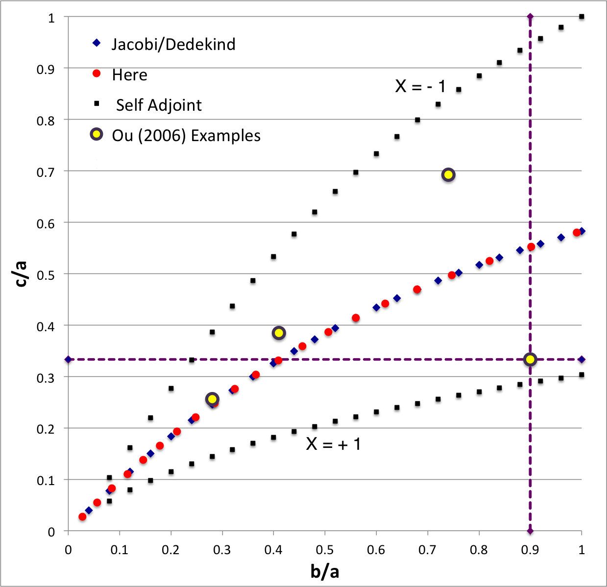
The model that we have chosen to use in our second successful construction of a COLLADA-based, 3D and interactive animation has the following properties; this model has been selected from [[User:Tohline/ThreeDimensionalConfigurations/RiemannStype#Table2|Table 2 of our accompanying discussion of Riemann S-type ellipsoids]]: | |||
<table border="0" cellpadding="5" align="center"> | |||
<tr> | |||
<td align="center" rowspan="6"> | |||
<b>Figure 1a</b><br /> <br /> | |||
[[File:B90c333EFEdiagram02.png|325px|EFE Parameter Space]] | |||
</td> | |||
<td align="center" rowspan="6" width="2%"> | |||
| |||
</td> | |||
<td align="center" colspan="3"> | |||
<math>~\frac{b}{a} = 0.90</math> | |||
</td> | |||
<td align="center" rowspan="6" width="2%"> | |||
| |||
</td> | |||
<td align="center" rowspan="6" bgcolor="lightgrey"> | |||
<b>Figure 1b</b><br /> | |||
[[File:COLLADAb90c333NewModel.png|300px|EFE Model b90c333]] | |||
</td> | |||
</tr> | |||
<tr> | |||
<td align="center" colspan="3"> | |||
<math>~\frac{c}{a} = 0.333</math> | |||
</td> | |||
</tr> | |||
<tr> | |||
<td align="center"> | |||
''Direct'' | |||
</td> | |||
<td align="center" width="2%" rowspan="4"> | |||
| |||
</td> | |||
<td align="center"> | |||
''Adjoint'' | |||
</td> | |||
</tr> | |||
<tr> | |||
<td align="center"> | |||
<math>~\Omega_\mathrm{EFE} = 0.447158</math> | |||
</td> | |||
<td align="center"> | |||
<math>~\Omega_\mathrm{EFE} = 0.221411</math> | |||
</td> | |||
</tr> | |||
<tr> | |||
<td align="center"> | |||
<math>~\lambda_\mathrm{EFE} = - 0.221411</math> | |||
</td> | |||
<td align="center"> | |||
<math>~\lambda_\mathrm{EFE} = - 0.447158 </math> | |||
</td> | |||
</tr> | |||
<tr> | |||
<td align="center"> | |||
<math>~f = + 0.995805</math> | |||
</td> | |||
<td align="center"> | |||
<math>~f = + 4.061607 </math> | |||
</td> | |||
</tr> | |||
</table> | |||
The subscript "EFE" on Ω and λ means that the relevant frequency is given in units that have been adopted in [<b>[[User:Tohline/Appendix/References#EFE|<font color="red">EFE</font>]]</b>], that is, in units of <math>~[\pi G\rho]^{1 / 2}</math>. In Figure 1a, the yellow circular marker, that has been placed where the pair of purple dashed lines cross, identifies the location of this model in the "c/a versus b/a" ''[[User:Tohline/ThreeDimensionalConfigurations/RiemannStype#Fig2|EFE Diagram]]'' that appears as Figure 2 on p. 902 of [http://adsabs.harvard.edu/abs/1965ApJ...142..890C S. Chandrasekhar (1965)]; essentially the same diagram appears in §49 (p. 147) of [<b>[[User:Tohline/Appendix/References#EFE|<font color="red">EFE</font>]]</b>]. | |||
===b74c692=== | |||
The model that we have chosen to use in our second successful construction of a COLLADA-based, 3D and interactive animation has the following properties; this model has been selected from [[User:Tohline/ThreeDimensionalConfigurations/RiemannStype#Table2|Table 2 of our accompanying discussion of Riemann S-type ellipsoids]]: | |||
<table border="0" cellpadding="5" align="center"> | |||
<tr> | <tr> | ||
<td align=" | <td align="center" rowspan="6"> | ||
[[File: | <b>Figure 1a</b><br /> <br /> | ||
</td> | [[File:B74c692EFEdiagram02.png|325px|EFE Parameter Space]] | ||
</td> | |||
<td align="center" rowspan="6" width="2%"> | |||
| |||
</td> | |||
<td align="center" colspan="3"> | |||
<math>~\frac{b}{a} = 0.74</math> | |||
</td> | |||
<td align="center" rowspan="6" width="2%"> | |||
| |||
</td> | |||
<td align="center" rowspan="6" bgcolor="lightgrey"> | |||
<b>Figure 1b</b><br /> | |||
[[File:COLLADAb74c692NewModel.png|300px|EFE Model b74c692]] | |||
</td> | |||
</tr> | |||
<tr> | |||
<td align="center" colspan="3"> | |||
<math>~\frac{c}{a} = 0.692</math> | |||
</td> | |||
</tr> | |||
<tr> | |||
<td align="center"> | |||
''Direct'' | |||
</td> | |||
<td align="center" width="2%" rowspan="4"> | |||
| |||
</td> | |||
<td align="center"> | |||
''Adjoint'' | |||
</td> | |||
</tr> | |||
<tr> | |||
<td align="center"> | |||
<math>~\Omega_\mathrm{EFE} = 0.638747</math> | |||
</td> | |||
<td align="center"> | |||
<math>~\Omega_\mathrm{EFE} = - 0.217773</math> | |||
</td> | |||
</tr> | |||
<tr> | |||
<td align="center"> | |||
<math>~\lambda_\mathrm{EFE} = 0.217773</math> | |||
</td> | |||
<td align="center"> | |||
<math>~\lambda_\mathrm{EFE} = - 0.638747 </math> | |||
</td> | |||
</tr> | |||
<tr> | |||
<td align="center"> | |||
<math>~f = - 0.713019</math> | |||
</td> | |||
<td align="center"> | |||
<math>~f = - 6.13413 </math> | |||
</td> | |||
</tr> | |||
</table> | |||
The subscript "EFE" on Ω and λ means that the relevant frequency is given in units that have been adopted in [<b>[[User:Tohline/Appendix/References#EFE|<font color="red">EFE</font>]]</b>], that is, in units of <math>~[\pi G\rho]^{1 / 2}</math>. In Figure 1a, the yellow circular marker, that has been placed where the pair of purple dashed lines cross, identifies the location of this model in the "c/a versus b/a" ''[[User:Tohline/ThreeDimensionalConfigurations/RiemannStype#Fig2|EFE Diagram]]'' that appears as Figure 2 on p. 902 of [http://adsabs.harvard.edu/abs/1965ApJ...142..890C S. Chandrasekhar (1965)]; essentially the same diagram appears in §49 (p. 147) of [<b>[[User:Tohline/Appendix/References#EFE|<font color="red">EFE</font>]]</b>]. | |||
===b28c256=== | |||
The model that we have chosen to use in our second successful construction of a COLLADA-based, 3D and interactive animation has the following properties; this model has been selected from [[User:Tohline/ThreeDimensionalConfigurations/RiemannStype#Table2|Table 2 of our accompanying discussion of Riemann S-type ellipsoids]]: | |||
<table border="0" cellpadding="5" align="center"> | |||
<tr> | |||
<td align="center" rowspan="6"> | |||
<b>Figure 1a</b><br /> <br /> | |||
[[File:B28c256EFEdiagram02.png|325px|EFE Parameter Space]] | |||
</td> | |||
<td align="center" rowspan="6" width="2%"> | |||
| |||
</td> | |||
<td align="center" colspan="3"> | |||
<math>~\frac{b}{a} = 0.28</math> | |||
</td> | |||
<td align="center" rowspan="6" width="2%"> | |||
| |||
</td> | |||
<td align="center" rowspan="6" bgcolor="lightgrey"> | |||
<b>Figure 1b</b><br /> | |||
[[File:COLLADAb28c256OldModel.png|300px|EFE Model b28c256]] | |||
</td> | |||
</tr> | |||
<tr> | |||
<td align="center" colspan="3"> | |||
<math>~\frac{c}{a} = 0.256</math> | |||
</td> | |||
</tr> | |||
<tr> | |||
<td align="center"> | |||
''Direct'' | |||
</td> | |||
<td align="center" width="2%" rowspan="4"> | |||
| |||
</td> | |||
<td align="center"> | |||
''Adjoint'' | |||
</td> | |||
</tr> | |||
<tr> | |||
<td align="center"> | |||
<math>~\Omega_\mathrm{EFE} = 0.456676</math> | |||
</td> | |||
<td align="center"> | |||
<math>~\Omega_\mathrm{EFE} = - 0.020692</math> | |||
</td> | |||
</tr> | |||
<tr> | |||
<td align="center"> | |||
<math>~\lambda_\mathrm{EFE} = 0.020692</math> | |||
</td> | |||
<td align="center"> | |||
<math>~\lambda_\mathrm{EFE} = - 0.456676</math> | |||
</td> | |||
</tr> | |||
<tr> | |||
<td align="center"> | |||
<math>~f = - 0.174510</math> | |||
</td> | |||
<td align="center"> | |||
<math>~f = - 85.0007</math> | |||
</td> | |||
</tr> | </tr> | ||
</table> | </table> | ||
The subscript "EFE" on Ω and λ means that the relevant frequency is given in units that have been adopted in [<b>[[User:Tohline/Appendix/References#EFE|<font color="red">EFE</font>]]</b>], that is, in units of <math>~[\pi G\rho]^{1 / 2}</math>. In Figure 1a, the yellow circular marker, that has been placed where the pair of purple dashed lines cross, identifies the location of this model in the "c/a versus b/a" ''[[User:Tohline/ThreeDimensionalConfigurations/RiemannStype#Fig2|EFE Diagram]]'' that appears as Figure 2 on p. 902 of [http://adsabs.harvard.edu/abs/1965ApJ...142..890C S. Chandrasekhar (1965)]; essentially the same diagram appears in §49 (p. 147) of [<b>[[User:Tohline/Appendix/References#EFE|<font color="red">EFE</font>]]</b>]. | |||
{{LSU_HBook_footer}} | {{LSU_HBook_footer}} | ||
Revision as of 21:16, 26 January 2021
For Shangli Ou

|
|---|
| | Tiled Menu | Tables of Content | Banner Video | Tohline Home Page | |
EFE Diagram
|
In the context of our broad discussion of ellipsoidal figures of equilibrium, the label "EFE Diagram" refers to a two-dimensional parameter space defined by the pair of axis ratios (b/a, c/a), usually covering the ranges, 0 ≤ b/a ≤ 1 and 0 ≤ c/a ≤ 1. The classic/original version of this diagram appears as Figure 2 on p. 902 of S. Chandrasekhar (1965, ApJ, vol. 142, pp. 890-921); a somewhat less cluttered version appears on p. 147 of Chandrasekhar's [EFE]. The version of the EFE Diagram shown here, on the left, highlights four model sequences, all of which also can be found in the original version:
Riemann S-type ellipsoids all lie between or on the two (self-adjoint) curves marked "X = -1" and "X = +1" in the EFE Diagram. The yellow circular markers in the diagram shown here, on the left, identify four Riemann S-type ellipsoids that were examined by Ou (2006) and that we have also chosen to use as examples. |
Example 3D Interactive Animations
b41c385
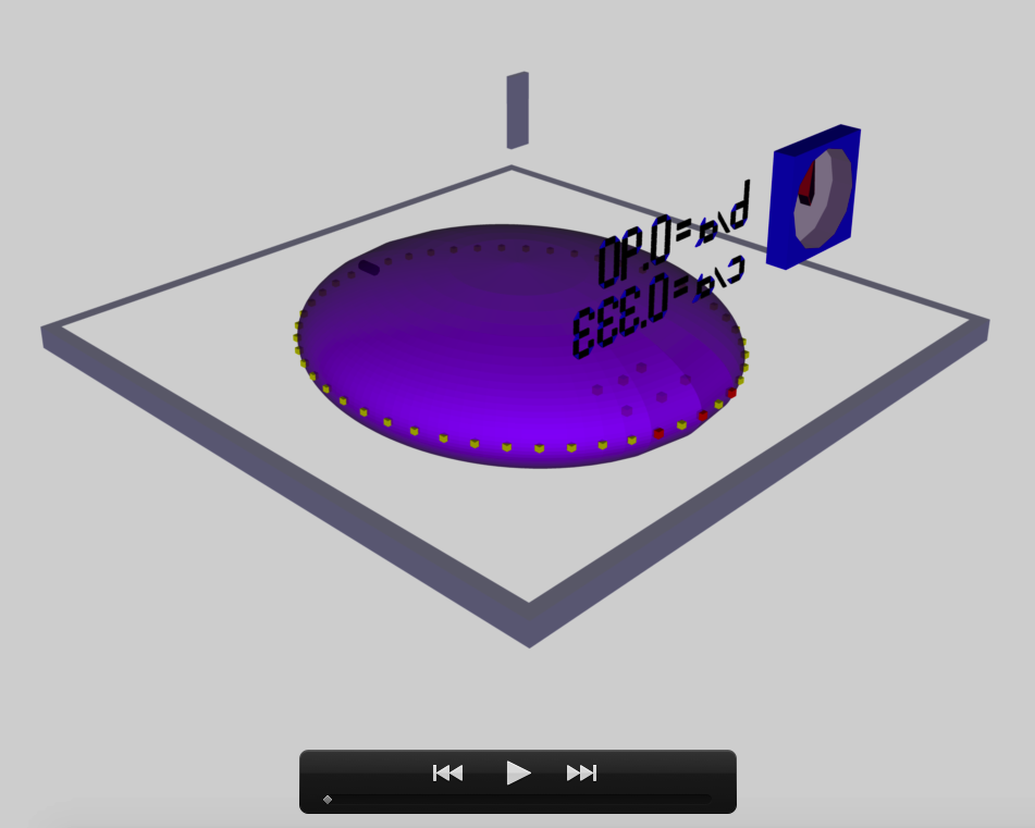
The model that we have chosen to use in our first successful construction of a COLLADA-based, 3D and interactive animation has the following properties; this model has been selected from Table 2 of our accompanying discussion of Riemann S-type ellipsoids:
|
|
<math>~\frac{b}{a} = 0.41</math> |
|
||||
|
<math>~\frac{c}{a} = 0.385</math> |
||||||
|
Direct |
|
Adjoint |
||||
|
<math>~\Omega_\mathrm{EFE} = 0.547874</math> |
<math>~\Omega_\mathrm{EFE} = - 0.079886</math> |
|||||
|
<math>~\lambda_\mathrm{EFE} = 0.079886</math> |
<math>~\lambda_\mathrm{EFE} = - 0.547874</math> |
|||||
|
<math>~f = - 0.415418</math> |
<math>~f = - 19.53923</math> |
|||||
The subscript "EFE" on Ω and λ means that the relevant frequency is given in units that have been adopted in [EFE], that is, in units of <math>~[\pi G\rho]^{1 / 2}</math>. In Figure 1a, the yellow circular marker, that has been placed where the pair of purple dashed lines cross, identifies the location of this model in the "c/a versus b/a" EFE Diagram that appears as Figure 2 on p. 902 of S. Chandrasekhar (1965); essentially the same diagram appears in §49 (p. 147) of [EFE].
In a separate chapter we have discussed various properties of uniformly rotating, Jacobi ellipsoids; they are equilibrium configurations that lie along the sequence that runs from "M2" (on the b/a = 1, Maclaurin sequence) to the origin of this diagram. Our chosen model lies off of — just above — the Jacobi-ellipsoid sequence, which means that it is not rotating as a solid body. Instead, as we focus first on the direct (as opposed to the adjoint) configuration, we appreciate that while the ellipsoid is spinning prograde (counter-clockwise) with a frequency given by |ΩEFE|, each Lagrangian fluid element inside as well as on the surface of the ellipsoid is traveling retrograde (clockwise) along an elliptical path with a frequency given by |λEFE|.
b90c333
The model that we have chosen to use in our second successful construction of a COLLADA-based, 3D and interactive animation has the following properties; this model has been selected from Table 2 of our accompanying discussion of Riemann S-type ellipsoids:
|
|
<math>~\frac{b}{a} = 0.90</math> |
|
||||
|
<math>~\frac{c}{a} = 0.333</math> |
||||||
|
Direct |
|
Adjoint |
||||
|
<math>~\Omega_\mathrm{EFE} = 0.447158</math> |
<math>~\Omega_\mathrm{EFE} = 0.221411</math> |
|||||
|
<math>~\lambda_\mathrm{EFE} = - 0.221411</math> |
<math>~\lambda_\mathrm{EFE} = - 0.447158 </math> |
|||||
|
<math>~f = + 0.995805</math> |
<math>~f = + 4.061607 </math> |
|||||
The subscript "EFE" on Ω and λ means that the relevant frequency is given in units that have been adopted in [EFE], that is, in units of <math>~[\pi G\rho]^{1 / 2}</math>. In Figure 1a, the yellow circular marker, that has been placed where the pair of purple dashed lines cross, identifies the location of this model in the "c/a versus b/a" EFE Diagram that appears as Figure 2 on p. 902 of S. Chandrasekhar (1965); essentially the same diagram appears in §49 (p. 147) of [EFE].
b74c692
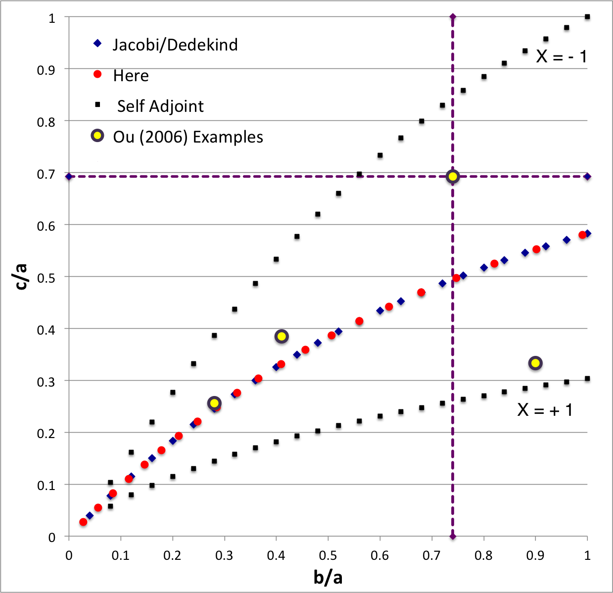
The model that we have chosen to use in our second successful construction of a COLLADA-based, 3D and interactive animation has the following properties; this model has been selected from Table 2 of our accompanying discussion of Riemann S-type ellipsoids:
|
|
<math>~\frac{b}{a} = 0.74</math> |
|
||||
|
<math>~\frac{c}{a} = 0.692</math> |
||||||
|
Direct |
|
Adjoint |
||||
|
<math>~\Omega_\mathrm{EFE} = 0.638747</math> |
<math>~\Omega_\mathrm{EFE} = - 0.217773</math> |
|||||
|
<math>~\lambda_\mathrm{EFE} = 0.217773</math> |
<math>~\lambda_\mathrm{EFE} = - 0.638747 </math> |
|||||
|
<math>~f = - 0.713019</math> |
<math>~f = - 6.13413 </math> |
|||||
The subscript "EFE" on Ω and λ means that the relevant frequency is given in units that have been adopted in [EFE], that is, in units of <math>~[\pi G\rho]^{1 / 2}</math>. In Figure 1a, the yellow circular marker, that has been placed where the pair of purple dashed lines cross, identifies the location of this model in the "c/a versus b/a" EFE Diagram that appears as Figure 2 on p. 902 of S. Chandrasekhar (1965); essentially the same diagram appears in §49 (p. 147) of [EFE].
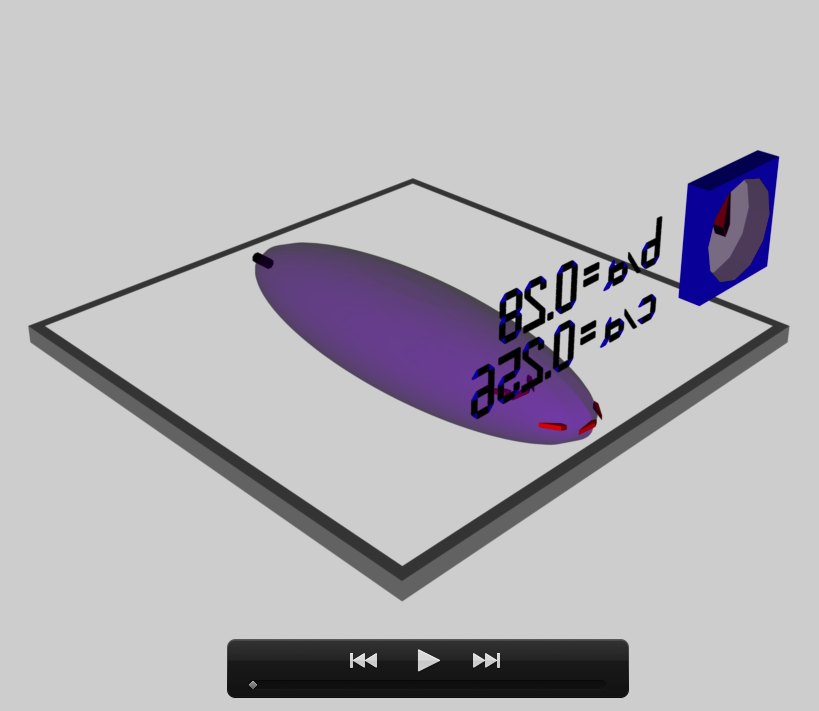
b28c256
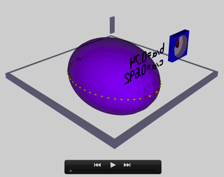
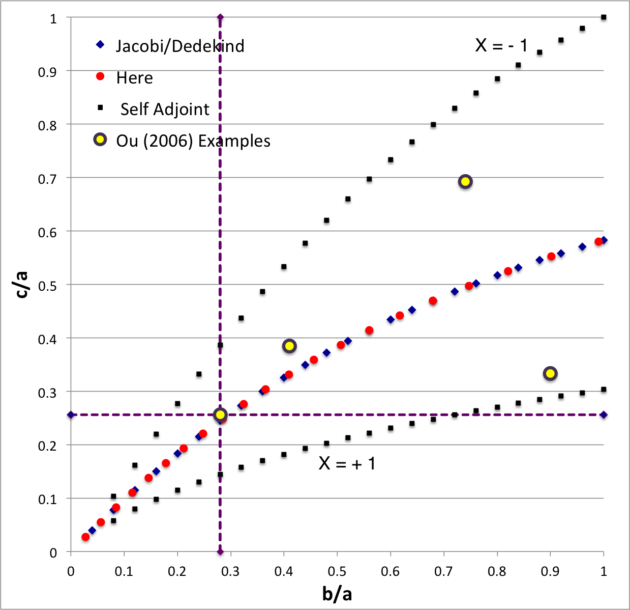
The model that we have chosen to use in our second successful construction of a COLLADA-based, 3D and interactive animation has the following properties; this model has been selected from Table 2 of our accompanying discussion of Riemann S-type ellipsoids:
|
|
<math>~\frac{b}{a} = 0.28</math> |
|
||||
|
<math>~\frac{c}{a} = 0.256</math> |
||||||
|
Direct |
|
Adjoint |
||||
|
<math>~\Omega_\mathrm{EFE} = 0.456676</math> |
<math>~\Omega_\mathrm{EFE} = - 0.020692</math> |
|||||
|
<math>~\lambda_\mathrm{EFE} = 0.020692</math> |
<math>~\lambda_\mathrm{EFE} = - 0.456676</math> |
|||||
|
<math>~f = - 0.174510</math> |
<math>~f = - 85.0007</math> |
|||||
The subscript "EFE" on Ω and λ means that the relevant frequency is given in units that have been adopted in [EFE], that is, in units of <math>~[\pi G\rho]^{1 / 2}</math>. In Figure 1a, the yellow circular marker, that has been placed where the pair of purple dashed lines cross, identifies the location of this model in the "c/a versus b/a" EFE Diagram that appears as Figure 2 on p. 902 of S. Chandrasekhar (1965); essentially the same diagram appears in §49 (p. 147) of [EFE].

|
|---|
|
© 2014 - 2021 by Joel E. Tohline |
