User:Tohline/Appendix/CGH/ParallelApertures

CGH: Apertures that are Parallel to the Image Screen

This chapter is intended primarily to replicate §I.A from the online class notes — see also an associated Preface and the original Table of Contents — that I developed in conjunction with a course that I taught in 1999 on the topic of Computer Generated Holography (CGH) for a subset of LSU physics majors who were interested in computational science.

Propagation of Light

Here we reference heavily the traveling, wave-like nature of light and, as is customary, use <math>~c</math> to represent its speed of propagation through space. Consider a single ray of light of wavelength, <math>~\lambda</math>, that is traveling in the <math>~x</math>-direction. Its amplitude, <math>~a</math>, will vary with time in a sinusoidal fashion as described by the equation,

<math>~a(x) = a_0\cos\biggl(\frac{2\pi x}{\lambda} + \phi_0 \biggr) \, ,</math>

where:  the light-wave's peak-to-peak brightness is <math>~2a_0</math>; <math>~\phi_0</math> is the "phase" that the oscillatory wave displays at a reference location, <math>~x=0</math>, when the reference time, <math>~t = 0</math>; and <math>~x = ct</math>. As is demonstrated, for example, in our accompanying discussion of various, equivalent, Fourier series expressions, this equation can be usefully rewritten in a number of other forms.

One-Dimensional Aperture

General Concept

Figure 1

Consider the amplitude (and phase) of light that is incident at a location <math>~y_1</math> on an image screen that is located a distance <math>~Z</math> from a slit of width <math>~w</math>. First, as illustrated in Figure 1, consider the contribution due only to two rays of light:  one coming from location <math>~Y_1</math> at the top edge of the slit (a distance <math>~D_1</math> from point <math>~y_1</math> on the screen) and another coming from location <math>~Y_2</math> at the bottom edge of the slit (a distance <math>~D_2</math> from the same point on the screen).

The complex number, <math>~A</math>, representing the light amplitude and phase at <math>~y_1</math> will be,

<math>~A(y_1)</math>

<math>~=</math>

<math>~ a(Y_1) e^{i(2\pi D_1/\lambda + \phi_1)} + a(Y_2) e^{i(2\pi D_2/\lambda + \phi_2)} \, , </math>

where, <math>~\lambda</math> is the wavelength of the light, <math>~a(Y_j)</math> is the brightness of the light at point <math>~Y_j</math> on the aperture, and <math>~\phi_j</math> is the phase of the light as it leaves point <math>~Y_j</math>.

Now, if we consider for the moment that at all locations on the aperture, <math>~Y_j</math>, the light has a brightness <math>~a(Y_j) = 1</math> and a phase <math>~\phi_j = 0</math>, then,

<math>~A(y_1)</math>

<math>~=</math>

<math>~A_0 \biggl[1 + e^{i(2\pi/\lambda)(D_2 - D_1)} \biggr] \, ,</math>

where, <math>~A_0 = e^{i(2\pi D_1/\lambda)}</math>. So the question of whether the amplitude at <math>~y_1</math> on the image screen will be bright due to constructive interference or faint as a result of destructive interference comes down to a question of what the phase difference is between the two distances <math>~D_1</math> and <math>~D_2</math> where,

<math>~D_j</math>	<math>~\equiv</math>	<math>~ [(Y_j - y_1)^2 + Z^2 ]^{1 / 2} </math>
	<math>~=</math>	<math>~ [Z^2 + y_1^2 - 2y_1 Y_j + Y_j^2 ]^{1 / 2} </math>
	<math>~=</math>	<math>~ L \biggl[1 - \frac{2y_1 Y_j}{L^2} + \frac{Y_j^2}{L^2} \biggr]^{1 / 2} </math>

and,

<math>~L</math>

<math>~\equiv</math>

<math>~ [Z^2 + y_1^2 ]^{1 / 2} \, . </math>

Utility of FFT Techniques

Let's rewrite the first of our above equations in a form that takes into account many more than just two points along the aperture. That is,

<math>~A(y_1)</math>	<math>~=</math>	<math>~\sum_j a_j e^{i(2\pi D_j/\lambda + \phi_j)} \, , </math>
	<math>~=</math>	<math>~\sum_j a_j \biggl[ \cos\biggl(\frac{2\pi D_j}{\lambda} + \phi_j \biggr) + i \sin\biggl(\frac{2\pi D_j}{\lambda} + \phi_j \biggr) \biggr] \, . </math>

Note that this is identical to the expression, <math>~A(y_1)</math> <math>~=</math> <math>~\sum_j a_j \biggl[\cos\phi_j + i \sin\phi_j \biggr] \biggl[ \cos\biggl(\frac{2\pi D_j}{\lambda} \biggr) + i \sin\biggl(\frac{2\pi D_j}{\lambda}\biggr) \biggr] \, . </math>

In the more restrictive case when we assume that everywhere along the aperture the phase <math>~\phi_j = 0</math>, we have,

<math>~A(y_1)</math>	<math>~=</math>	<math>~\sum_j a_j e^{i(2\pi D_j/\lambda)} \, , </math>
	<math>~=</math>	<math>~\sum_j a_j \biggl[ \cos\biggl(\frac{2\pi D_j}{\lambda} \biggr) + i \sin\biggl(\frac{2\pi D_j}{\lambda} \biggr) \biggr] \, , </math>

where, in each of these expressions, we have replaced <math>~a(Y_j)</math> with <math>~a_j</math>. After acknowledging that the function, <math>~A(y_1)</math>, is complex — with <math>~\mathcal{R}e(A)</math> being given by the sum over cosine terms and <math>~\mathcal{I}m(A)</math> being given by the sum over sine terms — it is clear that the brightness of each point on the image screen is given by (the square root of) <math>~A</math> multiplied by its complex conjugate, <math>~A^*</math>, that is, by the expression, <math>~ (A\cdot A^*)^{1 / 2}</math>. Figures 2 & 3 show how this brightness (amplitude) varies across the image screen for the case of a monochromatic light of wavelength, <math>~\lambda = 500</math> nanometers, impinging on a single slit that is 1 mm in width; for all curves, the amplitude has been determined by summing over <math>~j_\mathrm{max} = 51</math> equally spaced points across the slit. The results displayed in Figure 2 are for an image screen that is placed <math>~Z = 1</math> meter from the slit, while Figure 3 displays results for an image screen that is placed a distance, <math>~Z = 10</math> m from the slit.

Figure 2:   <math>~w = 1~\mathrm{mm}; Z = 1~\mathrm{m}; \lambda = 500~\mathrm{nm}; j_\mathrm{max} = 51</math>

Two curves appear in both Figure 2 and Figure 3. The solid green curve was obtained by plugging the precise, "nonlinear" determination of <math>~D_j</math> — that is, the mathematical expression for <math>~D_j</math>, as given above — into the arguments of the trigonometric functions, while the dotted red curve was obtained by using the approximate, "linearized" expression for <math>~D_j</math>, as will now be described.

Figure 3:   <math>~w = 1~\mathrm{mm}; Z = 10~\mathrm{m}; \lambda = 500~\mathrm{nm}; j_\mathrm{max} = 51</math>

If we assume that, for all <math>~j</math>,

<math>~\biggl| \frac{Y_j}{L}\biggr| \ll 1</math>

— in the present context, this generally will be equivalent to assuming that the width of the aperture is much much less than the distance <math>~(Z)</math> separating the aperture from the image screen — we can drop the quadratic term in favor of the linear one in the above expression for <math>~D_j</math> and deduce that,

<math>~D_j</math>	<math>~\approx</math>	<math>~ L \biggl[1 - \frac{2y_1 Y_j}{L^2} \biggr]^{1 / 2} </math>
	<math>~\approx</math>	<math>~ L \biggl[1 - \frac{y_1 Y_j}{L^2} \biggr] \, . </math>

Hence, we have,

<math>~A(y_1)</math>	<math>~\approx</math>	<math>~A_0 \sum_j a_j e^{-i[2\pi y_1 Y_j/(\lambda L)]} \, , </math>
	<math>~=</math>	<math>~A_0 \sum_j a_j \biggl[ \cos\biggl(\frac{2\pi y_1 Y_j}{\lambda L} \biggr) - i \sin\biggl(\frac{2\pi y_1 Y_j}{\lambda L} \biggr) \biggr] \, , </math>

where, now, <math>~A_0 = e^{i2\pi L/\lambda}</math>.

Notice that this expression matches what we have referred to elsewhere as the Complex Fourier Series Expression. When written in this form, it should immediately be apparent why discrete Fourier transform techniques (specifically FFT techniques) are useful tools for evaluation of the complex amplitude, <math>~A</math>. See further elaboration below.

Analytic Result

If we consider the limit where the aperture shown in Figure I.1 is divided into an infinite number of divisions, then we can convert the summation in the above equations into an integral running between the limits, Y₂ and Y₁. Specifically, linearized expression immediately above becomes,

<math>~A(y_1)</math>

<math>~\approx</math>

<math>~A_0~a_0 \int e^{-i[2\pi y_1 Y/(\lambda L)]} dY \, , </math>

where, again, we have returned to the case where the aperture is assumed to be uniformly bright and set a(Y) = a₀dY. (It should be understood that a₀ is the brightness of the aperture per unit length.) If we now make the substitution,

<math>~\Theta \equiv \frac{2\pi y_1 Y}{\lambda L} \, ,</math>

this integral expression takes the form,

<math>~A(y_1)</math>

<math>~\approx</math>

<math>~A_0 \biggl[ \frac{a_0 w}{2\beta_1} \biggr] \int_{\Theta_2}^{\Theta_1} e^{-i \Theta} d\Theta \, , </math>

where the limits of integration are, respectively,

<math>~\Theta_2</math>	<math>~\equiv</math>	<math>~ \frac{2\pi y_1 Y_2}{\lambda L} = \vartheta_1 - \beta_1 \, , </math>
<math>~\Theta_1</math>	<math>~\equiv</math>	<math>~ \frac{2\pi y_1 Y_1}{\lambda L} = \vartheta_1 + \beta_1 \, , </math>

and,

<math>~\beta_1</math>	<math>~\equiv</math>	<math>~ \frac{\pi y_1}{\lambda L} \biggl[ Y_1 - Y_2 \biggr] = \frac{\pi y_1 w}{\lambda L} \, , </math>
<math>~\vartheta_1</math>	<math>~\equiv</math>	<math>~ \frac{\pi y_1}{\lambda L} \biggl[ Y_1 + Y_2 \biggr] \, . </math>

This definite integral can be readily evaluated, giving,

<math>~A(y_1)</math>	<math>~\approx</math>	<math>~ (-i)^{-1} A_0 \biggl[ \frac{a_0 w}{2\beta_1} \biggr] \biggl[e^{-i\Theta_1} - e^{-i \Theta_2} \biggr] </math>
	<math>~=</math>	<math>~ i A_0 \biggl[ \frac{a_0 w}{2\beta_1} \biggr] e^{-i\vartheta_1} \biggl[e^{-i\beta_1} - e^{+i \beta_1} \biggr] </math>
	<math>~=</math>	<math>~ \biggl[ A_0 ~a_0 ~w ~e^{-i\vartheta_1} \biggr]\frac{\sin\beta_1}{\beta_1} = \biggl[ A_0 ~a_0 ~w ~e^{-i\vartheta_1} \biggr] \mathrm{sinc}(\beta_1) \, . </math>

The last two lines have been derived by realizing that, for any angle <math>~\chi</math>,

<math>~e^{-i\chi} - e^{+i\chi}</math>

<math>~=</math>

<math>~ -2i\sin(\chi) \, ; </math>

and the "sinc" function,

<math>~\mathrm{sinc}(\chi)</math>

<math>~=</math>

<math>~ \frac{\sin\chi}{\chi} \, . </math>

Notice that the center of the aperture is used to define the origin of the Y (and y) coordinate axis so that Y₂ = -Y₁, as illustrate in Figure I.1; then <math>~\vartheta_1 = 0</math> and the amplitude, A(y₁), has no complex component. If the aperture is not centered as depicted in Figure I.1, the angle <math>~\vartheta_1</math> simple serves to introduce a phase shift in the evaluation of the amplitude.

Although this problem was solved for a specific location, y₁, on the image screen, we see that the sinc function solution can readily be evaluated for any other location on the screen without having to redo the integral.

Location of the Dark Fringe(s)

As has been described in multiple online references, the locations across the image screen where complete destructive interference occurs can be determined straightforwardly using geometric relationships. For example, in terms of the angle, <math>~\theta</math>, defined such that,

<math>~\tan\theta = \frac{y_1}{Z} \, ,</math>

the distance from the central brightness peak to the first location where the brightness/amplitude goes to zero — i.e., the location of the first dark fringe — is given by the relation,

<math>~\sin\theta = \frac{\lambda}{w} \, .</math>

(For each successive fringe, labeled by the positive integer, <math>~m</math>, the relation is, <math>~\sin\theta_m = m\lambda/w.</math>) Hence, acknowledging that usually <math>~\lambda/w \ll 1</math>, we find that,

<math>~y_1\biggr|_{1^\mathrm{st} \mathrm{fringe}}</math>	<math>~=</math>	<math>~Z \tan\theta = Z \sin\theta [ 1 - \sin^2\theta ]^{-1 / 2}</math>
	<math>~=</math>	<math>~\frac{\lambda Z}{w} \biggl[ 1 - \biggl(\frac{\lambda }{w}\biggr)^2 \biggr]^{-1 / 2}</math>
	<math>~\approx</math>	<math>~\frac{\lambda Z}{w} \, .</math>

In the context of Figure 3, this means that, <math>~y_1|_{1^\mathrm{st} \mathrm{fringe}} = 5</math> millimeters, while, in Figure 2, <math>~y_1|_{1^\mathrm{st} \mathrm{fringe}} = 0.5</math> millimeters — in both cases, this is in agreement with the plotted linearized amplitude curves.

Parallels With Standard Fourier Series

Let's draw parallels between the above discussion of the single-slit diffraction pattern and our separate presentation of the standard treatment of Fourier Transforms.

Standard Fourier Transform Treatment	Single-Slit (Linearized) Diffraction Replace <math>~L</math> with <math>~\mathcal{D}</math>
<math>~a_m</math> <math>~=</math> <math>~ \frac{2}{L_\mathrm{max}} \cdot \sum_{L=1}^{L_\mathrm{max}} \rho(\theta_L) \cos\biggl[m \biggl(\frac{2\pi L}{L_\mathrm{max}}\biggr)\biggr] \, , </math> <math>~b_m</math> <math>~=</math> <math>~ \frac{2}{L_\mathrm{max}} \cdot \sum_{L=1}^{L_\mathrm{max}} \rho(\theta_L) \sin\biggl[m \biggl(\frac{2\pi L}{L_\mathrm{max}}\biggr)\biggr] \, . </math> It is sometimes useful to view <math>~a_m</math> and <math>~b_m</math> as, respectively, the real and imaginary components of a complex variable; for example, <math>~B(m)</math> <math>~=</math> <math>~a_m - i~b_m \, ,</math> in which case, Amplitude <math>~=</math> <math>~[a_m^2 + b_m^2]^{1 / 2} \, ,</math> Phase <math>~=</math> <math>~\tan^{-1}\biggl[\frac{-b_m}{a_m} \biggr]</math>	<math>~A(y_1)</math> <math>~=</math> <math>~A_0 \biggl[ \mathcal{R}e(A) - i ~\mathcal{I}m(A) \biggr] \, , </math> where, <math>~\mathcal{R}e[A(n\Delta y_1)]</math> <math>~=</math> <math>~\sum_j a_j \cos\biggl[n\Delta y_1 \biggl(\frac{2\pi}{\lambda \mathcal{D}} \biggr)j\Delta Y \biggr] \, , </math> <math>~\mathcal{I}m[A(n\Delta y_1)]</math> <math>~=</math> <math>~ \sum_j a_j \sin\biggl[n\Delta y_1 \biggl(\frac{2\pi}{\lambda \mathcal{D}} \biggr)j\Delta Y \biggr] \, . </math>
A comparison between the two discussions reveals the following variable mappings: <math>~m</math> <math>~\leftrightarrow</math> <math>~n</math> <math>~L</math> <math>~\leftrightarrow</math> <math>~j</math> <math>~\frac{2\pi}{L_\mathrm{max}}</math> <math>~\leftrightarrow</math> <math>~\Delta y_1 \biggl(\frac{2\pi}{\lambda \mathcal{D}} \biggr) \Delta Y </math> <math>~\rho(\theta_L)</math> <math>~\leftrightarrow</math> <math>~a(Y_j)</math>

---

Drawing from an accompanying discussion, the corresponding complex Fourier series expression is,

<math>~f(x)</math>

<math>~=</math>

<math>~ \frac{1}{2}\sum_{m = -\infty}^{m = + \infty} B(m) e^{i\omega_m x} \, , </math>

where, for <math>~m = 0, \pm 1, \pm 2, \pm 3, \dots~,</math>

<math>~\omega_m</math>

<math>~=</math>

<math>~ \frac{m\pi }{L} \, . </math>

In other words,

<math>~f(x)</math>	<math>~=</math>	<math>~ \frac{1}{2}\biggl[ B(m) e^{i\omega_m x}\biggr]_{m=0} + \frac{1}{2} \sum_{m = 1}^{m = + \infty} \biggl[ B(m) e^{i\omega_m x} + B(-m) e^{-i\omega_m x}\biggr] </math>
	<math>~=</math>	<math>~ \frac{B(0)}{2}\biggl[ \cos(\omega_m x) + i\sin(\omega_mx)\biggr]_{m=0} + \frac{1}{2} \sum_{m = 1}^{m = + \infty} \biggl\{ (a_m - ib_m)\biggl[ \cos(\omega_m x) + i\sin(\omega_mx)\biggr] + (a_m + ib_m) \biggl[ \cos(\omega_m x) - i\sin(\omega_mx)\biggr] \biggr\} </math>
	<math>~=</math>	<math>~ \frac{B(0)}{2} + \frac{1}{2} \sum_{m = 1}^{m = + \infty} \biggl\{ a_m \biggl[ \cos(\omega_m x) + i\sin(\omega_mx) \biggr] - ib_m \biggl[ \cos(\omega_m x) + i\sin(\omega_mx) \biggr] </math>
		<math>~ + a_m \biggl[ \cos(\omega_m x) - i\sin(\omega_mx)\biggr] + ib_m \biggl[ \cos(\omega_m x) - i\sin(\omega_mx)\biggr] \biggr\} </math>
	<math>~=</math>	<math>~ \frac{B(0)}{2} + \frac{1}{2} \sum_{m = 1}^{m = + \infty} \biggl\{ a_m \cos(\omega_m x) + i ~a_m \sin(\omega_mx) - i~b_m \cos(\omega_m x) + b_m\sin(\omega_mx) </math>
		<math>~ + a_m \cos(\omega_m x) - i~a_m\sin(\omega_mx) + ib_m \cos(\omega_m x) + b_m\sin(\omega_mx) \biggr\} </math>
	<math>~=</math>	<math>~ \frac{B(0)}{2} + \sum_{m = 1}^{m = + \infty} \biggl\{ a_m \cos(\omega_m x) + b_m\sin(\omega_mx) \biggr\} \, . </math>

---

Now, carry out the inverse transform.

Standard Fourier Transform Treatment	Single-Slit (Linearized) Diffraction Replace <math>~L</math> with <math>~\mathcal{D}</math>
<math>~\rho(\theta_L)</math> <math>~=</math> <math>~ \frac{a_0}{2} + \sum_{m=1}^{L_\mathrm{max}/2} \biggl\{ a_m \cos\biggl[m \biggl(\frac{2\pi L}{L_\mathrm{max}}\biggr)\biggr] + b_m\sin\biggl[m \biggl(\frac{2\pi L}{L_\mathrm{max}}\biggr)\biggr] \biggr\} </math>	<math>~a(Y_j)</math> <math>~=</math> <math>~ \frac{\mathcal{R}e(A_{n=0})}{2} + A_0 \sum_{n=1}^{n_\mathrm{max}/2} \biggl\{ \mathcal{R}e(A_n) \cos\biggl[n \biggl(\frac{2\pi j}{\lambda \mathcal{D}} \biggr)\Delta y_1 \Delta Y \biggr] + \mathcal{I}m(A_n)\sin\biggl[n\biggl(\frac{2\pi j}{\lambda \mathcal{D}} \biggr)\Delta y_1 \Delta Y \biggr] \biggr\} </math>

Parallels With Example #2

This "one dimensional aperture" analysis should exhibit features that strongly resemble the features that appear in our accompanying discussion of the Fourier series associated with a "square wave". In both cases — after performing both a Fourier transform and the inverse transform — the ultimate series expression that will represent the (square wave) amplitude across the aperture will take the form,

<math>~f(x)</math>

<math>~=</math>

<math>~ \frac{a_0}{2} + \sum_{n=1}^{\infty} \biggl[ a_n\cos \biggl(\frac{n\pi x}{L}\biggr) + b_n\sin \biggl(\frac{n\pi x}{L}\biggr) \biggr] \, . </math>

This function clearly repeats itself at spatial intervals of <math>~x \pm 2L</math>. Hence, we must acknowledge that, even if the initial state is intended to represent a single aperture, the inverse transform will produce an infinite set of identical apertures that are spaced (center-to-center) at intervals of <math>~2L</math>. We can presumably arrange to have successive apertures of width, <math>~2c</math>, widely spaced from one another by picking a value of <math>~|c/L | \ll 1</math>. (Reference, also, frame a of Figure 5, below, which depicts a uniformly illuminated (yellow), two-dimensional aperture whose horizontal width, as labeled, is <math>~2c_0 ;</math> the aperture has been cut into a mat of width, <math>~2L_0</math>.)

In the "square wave" analysis in which the brightness across the aperture is specified by a continuous function, the amplitude, <math>~a_n</math>, of each Fourier mode, <math>~n</math>, is given by the expression,

<math>~a_n</math>

<math>~=</math>

<math>~ \frac{1}{L} \int_{-c}^{c} \cos\biggl( \frac{n\pi x}{L} \biggr) dx = \biggl(\frac{2c}{L} \biggr) \mathrm{sinc}(\alpha_n)\, , </math>

where, <math>~\alpha_n \equiv n\pi c/L</math>. On the other hand, when a discrete Fourier transform is used, the analogous Fourier amplitude is given by the expression,

<math>~\mathcal{R}e[A(n\Delta y_1)]</math>

<math>~=</math>

<math>~\sum_{j=-j_\mathrm{max}}^{j_\mathrm{max}} \cos\biggl[n\Delta y_1 \biggl(\frac{2\pi}{\lambda \mathcal{D}} \biggr)\frac{j c}{j_\mathrm{max}} \biggr] \, . </math>

Comparing the two expressions, we recognize first that the integer, <math>~n</math>, has the same meaning in both; and, second, that <math>~x \leftrightarrow jc/j_\mathrm{max}</math>. Therefore — after recognizing that <math>~\mathcal{D} \approx Z</math> — it must also be true that,

<math>~\frac{1}{L} \leftrightarrow \frac{2\Delta y_1}{\lambda \mathcal{D}} \approx \frac{2\Delta y_1}{\lambda Z} \, .</math>

Next we notice, from the "square wave" analysis, that since the amplitude of the the diffraction pattern, <math>~a_n</math>, varies as <math>~\mathrm{sinc}(\alpha_n)</math>, the first dark fringe will arise when <math>~\alpha_n = \pi</math>, that is, when <math>~n = n_\pi \equiv L/c</math>. But, as explained above, from geometric arguments associated with the "one dimensional aperture" analysis, we expect the first dark fringe on the image screen to arise when,

<math>~\frac{y_1}{Z}</math>	<math>~=</math>	<math>~\frac{\lambda}{2c} </math>
<math>~\Rightarrow ~~~\frac{2}{\lambda Z}</math>	<math>~=</math>	<math>~\frac{1}{y_1 c} </math>
<math>~\Rightarrow ~~~\frac{\Delta y_1}{y_1 c} </math>	<math>~=</math>	<math>~\frac{2\Delta y_1}{\lambda Z} ~~\rightarrow ~~ \frac{1}{L} </math>
<math>~\Rightarrow ~~~n</math>	<math>~=</math>	<math>~ \frac{L}{c} ~~~\Rightarrow~~ n = n_\pi \, ,</math>

where this last relation has been derived by recognizing that, quite generally by design, <math>~y_1 = n\Delta y_1</math>. So, these two separate ways of identifying the location of the first dark fringe agree with one another.

COMMENT:   Throughout our discussion of computer-generated holography, we will find it necessary to construct a discretized image screen and, hence, will need to discuss the corresponding discretized modal amplitude ("sinc") function. This discretized amplitude function can be treated as a multiple-slit source function — reference, for example, frame c of Figure 5, below, which displays a 6 × 6 horizontal × vertical aperture layout — and, via an inverse Fourier transform, be used to regenerate the original square-wave (or analogous) function. This square wave of width, <math>~2c</math>, will necessarily be accompanied by multiple duplicate images that are spaced a (center-to-center) distance, <math>~2L</math>, apart. The result that we have just derived tells us that the relative spacing of these duplicate images will be large, relative to the width of the original square wave, if the discretization of the image screen is done in such a way as to ensure that <math>~n_\pi</math> is a large number.

More Attention to Detail

Theory

Guided by our accompanying discussion of the relationship between a one-dimensional aperture and the Fourier Series, let's begin again with the above general summation expression,

<math>~A(y_1)</math>	<math>~=</math>	<math>~\sum_j a_j e^{i(2\pi D_j/\lambda + \phi_j)} </math>
	<math>~\approx</math>	<math>~\sum_j a_j \mathrm{exp}\biggl\{i\biggl[ \frac{2\pi L_1}{\lambda} - \frac{2\pi y_1 Y_j}{L_1 \lambda} + \phi_j \biggr] \biggr\} </math>
	<math>~=</math>	<math>~\sum_j a_j \mathrm{exp}\biggl\{i\biggl[ \frac{2\pi L_1}{\lambda} - \frac{2\pi y_1 Y_0}{L_1 \lambda} - \frac{2\pi j y_1 \Delta Y}{L_1 \lambda} + \phi_j \biggr] \biggr\} </math>
	<math>~=</math>	<math>~\sum_j a_j \mathrm{exp}\biggl\{i\biggl[ \frac{2\pi L_1}{\lambda} - \frac{2\pi y_1 Y_0}{L_1 \lambda} + \phi_j \biggr] \biggr\} \biggl[ \cos\biggl(\frac{2\pi y_1 j \Delta Y}{\lambda L_1} \biggr) - i \sin\biggl(\frac{2\pi y_1 j \Delta Y}{\lambda L_1} \biggr) \biggr] </math>
	<math>~=</math>	<math>~ \mathrm{exp}\biggl\{i\biggl[ \frac{2\pi L_1}{\lambda} - \frac{2\pi y_1 Y_0}{L_1 \lambda} \biggr] \biggr\} \sum_j a_j e^{i\phi_j} \biggl[ \cos\biggl(\frac{2\pi y_1 j \Delta Y}{\lambda L_1} \biggr) - i \sin\biggl(\frac{2\pi y_1 j \Delta Y}{\lambda L_1} \biggr) \biggr] \, , </math>

where, <math>~0 \le j \le j_\mathrm{max}\, ,</math>

<math>~L_1</math>

<math>~\equiv</math>

<math>~[ Z^2 + y_1^2 ]^{1 / 2} \approx Z \biggl(1 + \frac{y_1^2}{2Z^2} \biggr) \, ,</math>

and we have inserted the following expression in order to identify discrete locations along the aperture,

<math>~Y_j</math>

<math>~=</math>

<math>~Y_0 + j\Delta Y = -\frac{w}{2} + j\biggl(\frac{w}{j_\mathrm{max}}\biggr) \, .</math>

Now, let's adopt the following conventions:

1. Specify the values of the parameters, <math>~\lambda, w, c/\mathfrak{L}_0,</math> and <math>~Z_0</math>, where,

   <math>~\mathfrak{L} \equiv \lambda Z j_\mathrm{max}/(2w) </math>     … hence …     <math>~\mathfrak{L}_0 = \lambda Z_0 j_\mathrm{max}/(2w) \, .</math>

2. In specifying the properties of the light as it leaves the aperture, ensure that neither <math>~a_j</math> nor <math>~\phi_j</math> depends on the distance between the aperture and the image plane, <math>~Z</math>.
3. It is best to evaluate the amplitude on the image screen over the range, <math>~-\mathfrak{L}_0 \le y_i \le \mathfrak{L}_0 \, .</math>
4. Expect the amplitude to be <math>~\sim 2c/\mathfrak{L}_0 \, .</math>

With this in mind, the expression for the image-screen amplitude can be rewritten as,

<math>~A(y_1)</math>	<math>~\approx</math>	<math>~ \mathrm{exp}\biggl\{i\biggl[ \frac{2\pi Z}{\lambda}\biggl(1 + \cancelto{0}{\frac{y_1^2}{2Z^2}} \biggr) + \frac{\pi y_1 w}{Z \lambda} \biggl( \cancelto{1}{\frac{Z}{L_1} } \biggr) \biggr] \biggr\} \sum_j a_j e^{i\phi_j} \biggl\{ \cos\biggl[ \frac{(\pi j y_1 ) 2w}{\lambda Z j_\mathrm{max}} \biggl( \cancelto{1}{\frac{Z}{L_1} } \biggr) \biggr] - i \sin\biggl[ \frac{(\pi j y_1 ) 2w}{\lambda Z j_\mathrm{max}} \biggl( \cancelto{1}{\frac{Z}{L_1} } \biggr) \biggr] \biggr\} </math>
	<math>~\approx</math>	<math>~ \mathrm{exp}\biggl\{i\biggl[ \frac{2\pi Z}{\lambda}+ \frac{\pi y_1 w}{Z \lambda} \biggr] \biggr\} \sum_j a_j e^{i\phi_j} \biggl\{ \cos\biggl( \frac{\pi j y_1 }{\mathfrak{L}} \biggr) - i \sin\biggl( \frac{\pi j y_1 }{\mathfrak{L}} \biggr) \biggr\} \, . </math>

First (Misguided) Attempt Next, let's set <math>~\phi_j = - 2\pi Z_0/\lambda</math>, which is independent of <math>~j</math> and therefore can be shifted outside of the summation. We have, then, <math>~A(y_1)</math> <math>~\approx</math> <math>~ \mathrm{exp}\biggl\{i\biggl[ \frac{2\pi (Z - Z_0)}{\lambda}+ \frac{\pi y_1 w}{Z \lambda} \biggr] \biggr\} \sum_j a_j \biggl\{ \cos\biggl( \frac{\pi j y_1 }{\mathfrak{L}} \biggr) - i \sin\biggl( \frac{\pi j y_1 }{\mathfrak{L}} \biggr) \biggr\} \, . </math>

Let's set,

<math>~\phi_j</math>

<math>~=</math>

<math>~- \frac{2\pi Z_0}{\lambda} - \frac{\pi y_1 w}{Z_0 \lambda} \, ,</math>

which is independent of <math>~j</math> and therefore can be shifted outside of the summation. We have, then,

<math>~A(y_1)</math>

<math>~\approx</math>

<math>~ \mathrm{exp}\biggl\{i\biggl[ \frac{2\pi (Z - Z_0)}{\lambda}+ \frac{\pi y_1 w}{Z \lambda} \biggr] \biggr\} \sum_j a_j \biggl\{ \cos\biggl( \frac{\pi j y_1 }{\mathfrak{L}} \biggr) - i \sin\biggl( \frac{\pi j y_1 }{\mathfrak{L}} \biggr) \biggr\} \, . </math>

Using this general expression, we should specifically expect the amplitude across the image plane at Z₀ to be a step function if we insert the expression,

<math>~a_j</math>

<math>~=</math>

<math>~\frac{2}{j \pi} \sin\biggl( \frac{j\pi c}{\mathfrak{L}_0} \biggr) = \biggl(\frac{2c}{\mathfrak{L}_0} \biggr) \mathrm{sinc}\biggl( \frac{j\pi c}{\mathfrak{L}_0} \biggr) \, .</math>

Hopefully, the amplitude of this image will die off quickly as we insert values of <math>~Z \ne Z_0 \, .</math>

Example #1

Let's try an example using the parameters listed at the top of Figure 4.

Figure 4:   <math>~w = 1~\mathrm{mm}; Z_0 = 10~\mathrm{m}; \lambda = 500~\mathrm{nm}; j_\mathrm{max} = 51</math>

Multiple One-Dimensional Apertures

Okay. Let's piece together an image that is generated by a set of <math>~N</math>, identical one-dimensional apertures; each one is uniformly illuminated, but adjacent apertures will, in general, have different illuminations, <math>~\beta_m</math>. Each aperture has width, <math>~2c</math>; and each is separated from its two neighboring apertures by a distance, <math>~2\nu</math>. (Reference frames b and c of Figure 5, below, which display, respectively, a 2 × 2 and 6 × 6 aperture-matrix layout in which all apertures are uniformly illuminated.)

Two Slits

Starting with just a pair of slits (as illustrated in frame b of Figure 5) and setting the x-direction zero point exactly midway between the two, we can expand upon the accompanying Example #2 discussion to obtain,

<math>~a_n</math>	<math>~=</math>	<math>~ \frac{1}{L} \biggl\{ \int_{\nu}^{\nu +2c} \beta_{+1} \cos\biggl( \frac{n\pi x}{L} \biggr) dx + \int^{-\nu}_{-(\nu +2c)} \beta_{-1}\cos\biggl( \frac{n\pi x}{L} \biggr) dx \biggr\} </math>
	<math>~=</math>	<math>~ \frac{1}{n\pi} \biggl\{ \int_{n\pi \nu/L}^{n\pi(\nu +2c)/L} \beta_{+1} \cos\theta ~d\theta + \int^{-n\pi \nu/L}_{-n\pi(\nu +2c)/L} \beta_{-1}\cos\theta ~d\theta \biggr\} </math>
	<math>~=</math>	<math>~ \frac{1}{n\pi} \biggl\{\beta_{+1} \biggl[ \sin\theta \biggr]_{n\pi \nu/L}^{n\pi(\nu +2c)/L} + \beta_{-1}\biggl[ \sin\theta \biggr]^{-n\pi \nu/L}_{-n\pi(\nu +2c)/L} \biggr\} </math>
	<math>~=</math>	<math>~ \frac{1}{n\pi} \biggl\{\beta_{+1} \biggl[ \sin\biggl( \frac{n\pi \nu }{L} + \frac{2n\pi c}{L}\biggr) - \sin\biggl( \frac{n\pi \nu}{L} \biggr) \biggr] + \beta_{-1}\biggl[\sin\biggl( -~\frac{n\pi \nu}{L} \biggr) - \sin\biggl( -~ \frac{n\pi \nu }{L} - \frac{2n\pi c}{L}\biggr) \biggr] \biggr\} </math>
	<math>~=</math>	<math>~ \frac{\beta_{+1} + \beta_{-1}}{n\pi} \biggl[ \sin\biggl( \frac{n\pi \nu }{L} + \frac{2n\pi c}{L}\biggr) - \sin\biggl( \frac{n\pi \nu}{L} \biggr) \biggr] \, ; </math>
<math>~b_n</math>	<math>~=</math>	<math>~ \frac{1}{n\pi} \biggl\{ \int_{n\pi \nu/L}^{n\pi(\nu +2c)/L} \beta_{+1} \sin\theta ~d\theta + \int^{-n\pi \nu/L}_{-n\pi(\nu +2c)/L} \beta_{-1}\sin\theta ~d\theta \biggr\} </math>
	<math>~=</math>	<math>~ \frac{1}{n\pi} \biggl\{ - \beta_{+1} \biggl[ \cos\theta\biggr]_{n\pi \nu/L}^{n\pi(\nu +2c)/L} - \beta_{-1} \biggl[ \cos\theta \biggr]^{-n\pi \nu/L}_{-n\pi(\nu +2c)/L} \biggr\} </math>
	<math>~=</math>	<math>~ \frac{1}{n\pi} \biggl\{ - \beta_{+1} \biggl[ \cos\biggl( \frac{n\pi \nu}{L} + \frac{2n\pi c}{L} \biggr) - \cos\biggl( \frac{n\pi\nu}{L} \biggr)\biggr] - \beta_{-1} \biggl[ \cos\biggl( - \frac{n\pi\nu}{L} \biggr) - \cos\biggl( -~\frac{n\pi\nu}{L} - ~\frac{2n\pi c}{L} \biggr) \biggr] \biggr\} </math>
	<math>~=</math>	<math>~-~ \frac{1}{n\pi} \biggl\{ \beta_{+1} \biggl[ \cos\biggl( \frac{n\pi \nu}{L} + \frac{2n\pi c}{L} \biggr) - \cos\biggl( \frac{n\pi\nu}{L} \biggr)\biggr] - \beta_{-1} \biggl[ \cos\biggl( \frac{n\pi\nu}{L} + \frac{2n\pi c}{L} \biggr) - \cos\biggl( \frac{n\pi\nu}{L} \biggr) \biggr] \biggr\} </math>
	<math>~=</math>	<math>~ \frac{\beta_{-1} - \beta_{+1}}{n\pi} \biggl[ \cos\biggl( \frac{n\pi \nu}{L} + \frac{2n\pi c}{L} \biggr) - \cos\biggl( \frac{n\pi\nu}{L} \biggr)\biggr] \, . </math>

Note that,

<math>~a_0</math>	<math>~=</math>	<math>~ \frac{1}{L} \biggl\{ \int_{\nu}^{\nu +2c} \beta_{+1} dx + \int^{-\nu}_{-(\nu +2c)} \beta_{-1} dx \biggr\} </math>
	<math>~=</math>	<math>~ \frac{1}{L} \biggl\{ \beta_{+1} \biggl[ \nu +2c - \nu \biggr] + \beta_{-1} \biggl[- \nu + (\nu +2c) \biggr] \biggr\} </math>
	<math>~=</math>	<math>~ \frac{2c(\beta_+ + \beta_-)}{L} \, . </math>

Considering, first, the case where the two slits are illuminated equally <math>(~\beta_- = \beta_+)</math>, we see that <math>~b_n = 0</math>, so the amplitude is,

<math>~|a_n|</math>	<math>~=</math>	<math>~ \frac{2}{n\pi} \biggl| \sin\biggl( \frac{n\pi \nu }{L} + \frac{2n\pi c}{L}\biggr) - \sin\biggl( \frac{n\pi \nu}{L} \biggr) \biggr| </math>
	<math>~=</math>	<math>~ \frac{2c}{L\chi_n} \biggl| \sin\biggl( \frac{\chi_n \nu }{c} + 2\chi_n \biggr) - \sin\biggl( \frac{\chi_n\nu}{c} \biggr) \biggr| </math>
	<math>~=</math>	<math>~ \frac{2c}{L\chi_n} \biggl| \sin\biggl[ \biggl( \frac{\chi_n\nu }{c} + \chi_n \biggr) + \chi_n \biggr] - \sin\biggl[ \biggl( \frac{\chi_n\nu }{c} + \chi_n \biggr) - \chi_n \biggr] \biggr| </math>
	<math>~=</math>	<math>~ \frac{4c}{L} \biggl| \cos\biggl[ \chi_n \biggl( 1 + \frac{\nu }{c} \biggr) \biggr] \frac{\sin \chi_n }{\chi_n} \biggr| \, , </math>

where,

<math>~\chi_n \equiv \frac{n\pi c}{L} \, .</math>

In the following animated figure, the red-dotted curve shows how <math>~\tfrac{L}{4c}|a_n|</math> varies with <math>~\chi_n/\pi</math> for a variety of values of the dimensionless parameter, <math>~0.01 \le \nu/c \le 5</math>, as recorded in the upper-right-hand corner of the plot.

Figure 4:  Double-Aperture Diffraction Pattern — Variable <math>~\nu/c</math>

The static, dashed-black curve in the figure displays the function,

<math>~\mathrm{sinc}(2\chi_n) = \frac{\sin(2\chi_n)}{2\chi_n} \, ,</math>

which is the proper amplitude behavior in the limit of <math>~\nu/c \rightarrow 0</math>. The static, solid black curve in the figure displays the function, <math>~\mathrm{sinc}(\chi_n)</math>; by inspection, this curve serves as the upper envelope to the amplitude function for all values of the dimensionless parameter, <math>~\nu/c</math>.

Two (or more) Slit Pairs

Now, let's examine four identical slits.

<math>~a_n</math>	<math>~=</math>	<math>~ \frac{1}{L} \biggl\{ \int_{(3\nu +2c)}^{(3\nu +4c)} \beta_{+2} \cos\biggl( \frac{n\pi x}{L} \biggr) dx + \int_{\nu}^{\nu +2c} \beta_{+1} \cos\biggl( \frac{n\pi x}{L} \biggr) dx + \int^{-\nu}_{-(\nu +2c)} \beta_{-1}\cos\biggl( \frac{n\pi x}{L} \biggr) dx + \int^{-(3\nu +2c)}_{-(3\nu + 4c)} \beta_{-2} \cos\biggl( \frac{n\pi x}{L} \biggr) dx \biggr\} </math>
	<math>~=</math>	<math>~ \frac{1}{n\pi} \biggl\{ \int_{n\pi(3\nu +2c)/L}^{n\pi(3\nu +4c)/L} \beta_{+2} \cos\theta ~ d\theta + \int_{n\pi\nu/L}^{n\pi(\nu +2c)/L} \beta_{+1} \cos\theta ~ d\theta + \int^{-n\pi \nu/L}_{-n\pi(\nu +2c)/L} \beta_{-1}\cos\theta ~d\theta + \int^{-n\pi (3\nu +2c)/L}_{-n\pi (3\nu + 4c)/L} \beta_{-2} \cos\theta~ d\theta \biggr\} </math>
	<math>~=</math>	<math>~ \frac{1}{n\pi} \biggl\{ \beta_{+2} \biggl[ \sin\theta \biggr]_{n\pi(3\nu +2c)/L}^{n\pi(3\nu +4c)/L} + \beta_{+1} \biggl[ \sin\theta \biggr]_{n\pi \nu/L}^{n\pi(\nu +2c)/L} + \beta_{-1}\biggl[ \sin\theta \biggr]^{-n\pi \nu/L}_{-n\pi(\nu +2c)/L} + \beta_{-2}\biggl[ \sin\theta \biggr]^{-n\pi (3\nu +2c)/L}_{-n\pi (3\nu + 4c)/L} \biggr\} </math>
	<math>~=</math>	<math>~ \frac{1}{n\pi} \biggl\{\beta_{+2} \biggl[ \sin\biggl( \frac{3n\pi \nu }{L} + \frac{4n\pi c}{L}\biggr) - \sin\biggl( \frac{3n\pi \nu }{L} + \frac{2n\pi c}{L} \biggr) \biggr] + \beta_{-2}\biggl[\sin\biggl( -~ \frac{3n\pi \nu }{L} - \frac{2n\pi c}{L}\biggr) - \sin\biggl( -~ \frac{3n\pi \nu }{L} - \frac{4n\pi c}{L}\biggr) \biggr] </math>
		<math>~ + \beta_{+1} \biggl[ \sin\biggl( \frac{n\pi \nu }{L} + \frac{2n\pi c}{L}\biggr) - \sin\biggl( \frac{n\pi \nu}{L} \biggr) \biggr] + \beta_{-1}\biggl[\sin\biggl( -~\frac{n\pi \nu}{L} \biggr) - \sin\biggl( -~ \frac{n\pi \nu }{L} - \frac{2n\pi c}{L}\biggr) \biggr] \biggr\} </math>
	<math>~=</math>	<math>~ \frac{1}{n\pi} \biggl\{ (\beta_{+2} + \beta_{-2}) \biggl[ \sin\biggl( \frac{3n\pi \nu }{L} + \frac{4n\pi c}{L}\biggr) - \sin\biggl( \frac{3n\pi \nu }{L} + \frac{2n\pi c}{L} \biggr) \biggr] + (\beta_{+1}+ \beta_{-1}) \biggl[ \sin\biggl( \frac{n\pi \nu }{L} + \frac{2n\pi c}{L}\biggr) - \sin\biggl( \frac{n\pi \nu}{L} \biggr) \biggr] \biggr\} </math>
	<math>~=</math>	<math>~ \frac{(\beta_{+2} + \beta_{-2})}{n\pi} \biggl\{ \sin\biggl[ \frac{n\pi }{L} \biggr( 3\nu + 4c \biggr) \biggr] - \sin\biggl[ \frac{n\pi }{L} \biggr( 3\nu + 2c \biggr) \biggr] \biggr\} + \frac{(\beta_{+1}+ \beta_{-1})}{n\pi} \biggl\{ \sin\biggl[ \frac{n\pi }{L} \biggr( \nu + 2c \biggr) \biggr] - \sin\biggl[ \frac{n\pi }{L} \biggr( \nu \biggr)\biggr] \biggr\} \, . </math>

Note that,

<math>~a_0</math>	<math>~=</math>	<math>~ \frac{1}{L} \biggl\{ \int_{ (3\nu +2c)}^{ (3\nu +4c)} \beta_{+2} dx + \int_{\nu}^{\nu +2c} \beta_{+1} dx + \int^{-\nu}_{-(\nu +2c)} \beta_{-1} dx + \int^{-(3\nu +2c)}_{-(3\nu + 4c)} \beta_{-2} dx \biggr\} </math>
	<math>~=</math>	<math>~ \frac{1}{L} \biggl\{ \beta_{+2} \biggl[ (3\nu +4c) - (3\nu +2c) \biggr] + \beta_{+1} \biggl[ \nu +2c - \nu \biggr] + \beta_{-1} \biggl[- \nu + (\nu +2c) \biggr] + \beta_{-2} \biggl[-(3\nu +2c) + (3\nu + 4c) \biggr] \biggr\} </math>
	<math>~=</math>	<math>~ \frac{ 2c(\beta_{-2} + \beta_{-1} + \beta_{+1} + \beta_{+2} ) }{L} \, . </math>

Therefore, for an arbitrary number of slit pairs, <math>~j_\mathrm{slits}</math>, it appears as though,

<math>~a_n</math>	<math>~=</math>	<math>~\sum_{j=1}^{j_\mathrm{slits}} \frac{(\beta_{+j} + \beta_{-j})}{n\pi} \biggl\{ \sin\biggl\{ \frac{n\pi }{L} \biggr[ (2j-1)(\nu + c) + c \biggr] \biggr\} - \sin\biggl\{ \frac{n\pi }{L} \biggr[ (2j-1)(\nu + c) - c \biggr] \biggr\} \biggr\} </math>
	<math>~=</math>	<math>~\sum_{j=1}^{j_\mathrm{slits}} \frac{2(\beta_{+j} + \beta_{-j})}{n\pi} \biggl\{ \cos\biggl[ \frac{n\pi (2j-1)(\nu + c) }{L} \biggr] \sin\biggl[ \frac{n\pi c}{L} \biggr] \biggr\} </math>
	<math>~=</math>	<math>~\sum_{j=1}^{j_\mathrm{slits}} \frac{2c(\beta_{+j} + \beta_{-j})}{L} \biggl\{ \cos \biggl[ \chi_n(2j-1)\biggl( 1 + \frac{\nu}{c} \biggr) \biggr] \frac{\sin\chi_n}{\chi_n} \biggr\} </math>
	<math>~=</math>	<math>~\frac{2c}{L} \cdot \frac{\sin\chi_n}{\chi_n} ~\sum_{j=1}^{j_\mathrm{slits}} (\beta_{+j} + \beta_{-j}) \cos \biggl[ \chi_n(2j-1)\biggl( 1 + \frac{\nu}{c} \biggr) \biggr] \, , </math>

where, as before, <math>~\chi_n \equiv (n\pi c/L)</math>, with the special case,

<math>~a_0</math>

<math>~=</math>

<math>~\frac{2c}{L} \sum_{j=1}^{j_\mathrm{slits}} \biggl[ \beta_{+j} + \beta_{-j} \biggr] \, . </math>

Behavior of <math>~a_n</math> when <math>~\beta_{\pm j} = 1</math> for all <math>~j</math>, and in the limit, <math>~\frac{\nu}{c} \rightarrow 0</math>.

When <math>~j_\mathrm{slits} = 1</math>: <math>~a_n</math> <math>~=</math> <math>~\frac{2c}{L} \cdot \frac{\sin\chi_n}{\chi_n} \cdot (2) \cos \chi_n </math>   <math>~=</math> <math>~\frac{4c}{L} \cdot \frac{\sin(2\chi_n)}{(2\chi_n)} </math> When <math>~j_\mathrm{slits} = 2</math>: <math>~a_n</math> <math>~=</math> <math>~\frac{2c}{L} \cdot \frac{\sin\chi_n}{\chi_n} ~\biggl\{ \sum_{j=1}^{2} (2) \cos \biggl[ \chi_n(2j-1) \biggr] \biggr\} </math>   <math>~=</math> <math>~\frac{4c}{L} \cdot \frac{\sin\chi_n}{\chi_n} ~\biggl\{ \cos \chi_n + \cos (3\chi_n ) \biggr\} </math>   <math>~=</math> <math>~\frac{4c}{L} \cdot \frac{\sin\chi_n}{\chi_n} ~\biggl\{ \cos \chi_n + 4\cos^3\chi_n -3\cos\chi_n \biggr\} </math>   <math>~=</math> <math>~\frac{4c}{L} \cdot \frac{\sin\chi_n \cos\chi_n}{\chi_n} ~\biggl\{ 4\cos^2\chi_n - 2 \biggr\} </math>   <math>~=</math> <math>~\frac{4c}{L} \cdot \frac{\sin\chi_n \cos\chi_n}{\chi_n} ~\biggl\{ 2 - 4\sin^2\chi_n \biggr\} </math>   <math>~=</math> <math>~\frac{8c}{L} \cdot \frac{\sin(4\chi_n )}{(4\chi_n)} \, . </math> When <math>~j_\mathrm{slits} = 3</math>: <math>~a_n</math> <math>~=</math> <math>~\frac{4c}{L} \cdot \frac{\sin\chi_n}{\chi_n} ~\biggl\{ \sum_{j=1}^{3} \cos \biggl[ \chi_n(2j-1) \biggr] \biggr\} </math>   <math>~=</math> <math>~\frac{4c}{L} \cdot \frac{\sin\chi_n}{\chi_n} ~\biggl\{ \cos \chi_n + \cos (3\chi_n ) + \cos (5\chi_n) \biggr\} </math>   <math>~=</math> <math>~\frac{4c}{L} \cdot \frac{\sin\chi_n}{\chi_n} ~\biggl\{ \cos \chi_n + [ 4\cos^3\chi_n - 3\cos\chi_n ] + [ 16\cos^5\chi_n -20\cos^3\chi_n + 5\cos\chi_n ] \biggr\} </math>   <math>~=</math> <math>~\frac{4c}{L} \cdot \frac{\sin\chi_n \cos\chi_n}{\chi_n} ~\biggl\{ 3 -16\cos^2\chi_n + 16\cos^4\chi_n \biggr\} </math>   <math>~=</math> <math>~\frac{12c}{L} \cdot \frac{\sin(6\chi_n) }{6\chi_n} </math> Therefore, it appears as though, for arbitrary values of <math>~j_\mathrm{slits} \ge 1</math>, <math>~a_n</math> <math>~=</math> <math>~\frac{4 j_\mathrm{slits}c}{L} \cdot \frac{\sin(2j_\mathrm{slits}\chi_n) }{(2 j_\mathrm{slits}\chi_n)} </math> <math>~=</math> <math>~\frac{(2c)(2 j_\mathrm{slits})}{L} \cdot \mathrm{sinc} (2j_\mathrm{slits}\chi_n) </math> I have not yet proven that the above, generalized expression for <math>~a_n</math> works for all values of <math>~j_\mathrm{slits}</math>. To do so will likely involve enlisting the following two generalized trigonometric (Multiple-angle) relations that appear on p. 190 of my CRC handbook of Standard Mathematical Tables. <math>~\sin(n\alpha)</math> <math>~=</math> <math>~ 2\sin[(n-1)\alpha] \cos\alpha - \sin[(n-2)\alpha] \, , </math> <math>~\cos(n\alpha)</math> <math>~=</math> <math>~ 2\cos[(n-1)\alpha] \cos\alpha - \cos[(n-2)\alpha] \, . </math>

VARIOUS SCALINGS:

1. Given that <math>~\beta</math> has units of brightness per unit length, with <math>~\beta_0</math> referring to the brightness per unit length that is incident on the single slit; and, given that in the above formulation each separate slit has a width of <math>~2c</math>, the total brightness emerging from a uniformly illuminated multi-slit configuration is,

   <math>~b_\mathrm{tot} = 2j_\mathrm{slits}(2c\beta_0) \, .</math>

   Hence, in order for every configuration's total brightness to be the same — that is, to be equal to <math>~2c_0\beta_0,</math> where <math>~c_0</math> is the half-width of the single slit — in each case we need to set <math>~c \rightarrow c_0/(2j_\mathrm{slits})</math>.

2. As is illustrated by frame a of Figure 5, below, the total width of the single slit is <math>~2c_0</math>, while — see frames b and c of Figure 5 — the total width of the combined slit(s) is

   <math>~C_\mathrm{tot} = (2j_\mathrm{slits})2c + (2j_\mathrm{slits}-1)2\nu \, .</math>

   Hence, if we want the ratio of the slit width to the Fourier width, <math>~2L</math>, to be the same for each multi-slit example, in each case we need to set,

   <math>~\frac{C_\mathrm{tot}}{2L}</math>	<math>~=</math>	<math>~\frac{c_0}{L_0}</math>
   <math>~\Rightarrow ~~~ L \rightarrow \frac{L_0 C_\mathrm{tot}}{2c_0} </math>	<math>~=</math>	<math>~\frac{L_0 }{c_0} \biggl[ (2j_\mathrm{slits})c + (2j_\mathrm{slits} -1) \nu \biggr]</math>

   Or, put together, we have,

   <math>~ L </math>

   <math>~\rightarrow</math>

   <math>~L_0 \biggl[ 1 + \frac{(2j_\mathrm{slits} -1) \nu}{ (2j_\mathrm{slits})c}\biggr]</math>

 

Figure 5
Frame a:  Single Aperture Frame b:  Double Aperture <math>~(j_\mathrm{slits} = 1)</math> Frame c:  Multiple Apertures <math>~(j_\mathrm{slits} = 3)</math>

Incorporating these normalizations, we have,

<math>~a_n</math>

<math>~=</math>

<math>~\frac{c_0}{j_\mathrm{slits} L_0} \biggl[ 1 + \frac{(2j_\mathrm{slits} -1) \nu}{ (2j_\mathrm{slits})c}\biggr]^{-1} \frac{\sin\chi_n}{\chi_n} ~\sum_{j=1}^{j_\mathrm{slits}} (\beta_{+j} + \beta_{-j}) \cos \biggl[ \chi_n(2j-1)\biggl( 1 + \frac{\nu}{c} \biggr) \biggr] \, , </math>

and,

<math>~a_0</math>

<math>~=</math>

<math>~\frac{c_0}{j_\mathrm{slits} L_0} \biggl[ 1 + \frac{(2j_\mathrm{slits} -1) \nu}{ (2j_\mathrm{slits})c}\biggr]^{-1} \sum_{j=1}^{j_\mathrm{slits}} \biggl[ \beta_{+j} + \beta_{-j} \biggr] \, , </math>

where,

<math>~\chi_n \equiv \frac{n\pi c}{L}</math>

<math>~=</math>

<math>~\frac{n \pi c_0}{ 2 j_\mathrm{slits} L_0} \biggl[ 1 + \frac{(2j_\mathrm{slits} -1) \nu}{ (2j_\mathrm{slits})c}\biggr]^{-1} \, . </math>

Figure 6
<math>~\frac{c_0}{L_0} = \frac{1}{20} </math>     and     <math>~\frac{\nu}{c} = \frac{1}{10}</math>    for various <math>~j_\mathrm{slits}</math>

---

By generalizing, we also see that,

<math>~b_n</math>	<math>~=</math>	<math>~ \frac{1}{n\pi} \biggl\{ \int_{n\pi \nu/L}^{n\pi(\nu +2c)/L} \beta_{+1} \sin\theta ~d\theta + \int^{-n\pi \nu/L}_{-n\pi(\nu +2c)/L} \beta_{-1}\sin\theta ~d\theta \biggr\} </math>
	<math>~=</math>	<math>~ \frac{1}{n\pi} \biggl\{ - \beta_{+1} \biggl[ \cos\theta\biggr]_{n\pi \nu/L}^{n\pi(\nu +2c)/L} - \beta_{-1} \biggl[ \cos\theta \biggr]^{-n\pi \nu/L}_{-n\pi(\nu +2c)/L} \biggr\} </math>
	<math>~=</math>	<math>~ \frac{1}{n\pi} \biggl\{ - \beta_{+1} \biggl[ \cos\biggl( \frac{n\pi \nu}{L} + \frac{2n\pi c}{L} \biggr) - \cos\biggl( \frac{n\pi\nu}{L} \biggr)\biggr] - \beta_{-1} \biggl[ \cos\biggl( - \frac{n\pi\nu}{L} \biggr) - \cos\biggl( -~\frac{n\pi\nu}{L} - ~\frac{2n\pi c}{L} \biggr) \biggr] \biggr\} </math>
	<math>~=</math>	<math>~-~ \frac{1}{n\pi} \biggl\{ \beta_{+1} \biggl[ \cos\biggl( \frac{n\pi \nu}{L} + \frac{2n\pi c}{L} \biggr) - \cos\biggl( \frac{n\pi\nu}{L} \biggr)\biggr] - \beta_{-1} \biggl[ \cos\biggl( \frac{n\pi\nu}{L} + \frac{2n\pi c}{L} \biggr) - \cos\biggl( \frac{n\pi\nu}{L} \biggr) \biggr] \biggr\} </math>
	<math>~=</math>	<math>~ \frac{\beta_{-1} - \beta_{+1}}{n\pi} \biggl[ \cos\biggl( \frac{n\pi \nu}{L} + \frac{2n\pi c}{L} \biggr) - \cos\biggl( \frac{n\pi\nu}{L} \biggr)\biggr] \, . </math>

Considering, first, the case where the two slits are illuminated equally <math>(~\beta_- = \beta_+)</math>, we see that <math>~b_n = 0</math>, so the amplitude is,

<math>~|a_n|</math>	<math>~=</math>	<math>~ \frac{2}{n\pi} \biggl| \sin\biggl( \frac{n\pi \nu }{L} + \frac{2n\pi c}{L}\biggr) - \sin\biggl( \frac{n\pi \nu}{L} \biggr) \biggr| </math>
	<math>~=</math>	<math>~ \frac{2c}{L\chi} \biggl| \sin\biggl( \frac{\chi\nu }{c} + 2\chi \biggr) - \sin\biggl( \frac{\chi\nu}{c} \biggr) \biggr| \, , </math>

where,

<math>~\chi \equiv \frac{n\pi c}{L} \, .</math>

Check List

Here is a list of issues that need to be discussed/explained in order to establish a foundation for the topic of this chapter.

1. Huygens-Fresnel Principle
1. Single Aperture (or Reflecting Surface)
1. Exact Representation

   <math>~A(y_1)</math>	<math>~=</math>	<math>~\sum_j a_j e^{i(2\pi D_j/\lambda + \phi_j)} \, , </math>
   	<math>~=</math>	<math>~\sum_j a_j \biggl[\cos\phi_j + i \sin\phi_j \biggr] \biggl[ \cos\biggl(\frac{2\pi D_j}{\lambda} \biggr) + i \sin\biggl(\frac{2\pi D_j}{\lambda}\biggr) \biggr] \, , </math>
   where …    <math>~D_j</math>	<math>~=</math>	<math>~ \mathcal{L} \biggl[1 - \frac{2y_1 Y_j}{\mathcal{L}^2} + \frac{Y_j^2}{\mathcal{L}^2} \biggr]^{1 / 2} </math>     and     <math>~ \mathcal{L} \equiv [Z^2 + y_1^2 ]^{1 / 2} \, . </math>

2. Approximation
   Realizing that,

   <math>~\frac{2\pi D_j}{\lambda}</math>	<math>~\approx</math>	<math>~ \biggl[\frac{2\pi \mathcal{L}}{\lambda} - \frac{2\pi y_1 Y_j}{\lambda \mathcal{L}} \biggr] </math>
   <math>~\Rightarrow ~~~ A(y_1)</math>	<math>~\approx</math>	<math>~e^{i(2\pi \mathcal{L}/\lambda)} \cdot \sum_j a_j e^{i \phi_j } \cdot e^{-i(2\pi y_1 Y_j/\lambda \mathcal{L})} \, , </math>
   	<math>~=</math>	<math>~e^{i(2\pi \mathcal{L}/\lambda)} \cdot \sum_j a_j \biggl[\cos\phi_j + i \sin\phi_j \biggr] \biggl[ \cos\biggl(\frac{2\pi y_1 Y_j}{\lambda \mathcal{L}} \biggr) - i \sin\biggl(\frac{2\pi y_1 Y_j}{\lambda \mathcal{L}} \biggr) \biggr] \, . </math>

2. Double Aperture
   

   Here, on the right, we have replicated frame b from Figure 5, which displays four yellow square apertures — each of width, <math>~2c</math>, as indicated — arranged in a 2 × 2 matrix on a background mat of width, <math>~2L</math>. The apertures are separated horizontally from each other by a distance, <math>~2\nu</math>, so, as illustrated, the distance from the center of the mat to the outer edge of an aperture is <math>~(\nu + 2c)</math>. Referencing only the horizontal layout of apertures in this image — that is, ignoring its vertical layout to focus on the simpler, one-dimensional problem — we see that the image represents a single pair of apertures and, hence, the case (referenced below) where <math>~j_\mathrm{slits} = 1</math>.

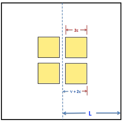
   Making the substitutions,

   <math>~Y_j ~\rightarrow ~x</math>       and       <math>\frac{2y_1}{\lambda \mathcal{L}}~\rightarrow ~\frac{n}{L}</math>
   <math>~\Rightarrow ~~~ a_n</math>	<math>~=</math>	<math>~ \frac{1}{L} \biggl\{ \int_{\nu}^{\nu +2c} \beta_{+1} \cos\biggl( \frac{n\pi x}{L} \biggr) dx + \int^{-\nu}_{-(\nu +2c)} \beta_{-1}\cos\biggl( \frac{n\pi x}{L} \biggr) dx \biggr\} </math>
   	<math>~=</math>	<math>~ \frac{\beta_{+1} + \beta_{-1}}{n\pi} \biggl[ \sin\biggl( \frac{n\pi \nu }{L} + \frac{2n\pi c}{L}\biggr) - \sin\biggl( \frac{n\pi \nu}{L} \biggr) \biggr] </math>
   	<math>~=</math>	<math>~ \frac{\beta_{+1} + \beta_{-1}}{n\pi} \biggl\{ \sin \biggl[ \biggl( \frac{n\pi \nu }{L} + \frac{n\pi c}{L}\biggr) + \frac{n\pi c}{L} \biggr] - \sin\biggl[ \biggl( \frac{n\pi \nu}{L} + \frac{n\pi c}{L} \biggr) - \frac{n\pi c}{L}\biggr] \biggr\} </math>
   	<math>~=</math>	<math>~ \frac{\beta_{+1} + \beta_{-1}}{n\pi} \biggl\{ 2 \cos \biggl[ \biggl( \frac{n\pi \nu }{L} + \frac{n\pi c}{L}\biggr) \biggr] \sin\biggl[ \frac{n\pi c}{L}\biggr] \biggr\} </math>
   	<math>~=</math>	<math>~ \frac{\beta_{+1} + \beta_{-1}}{n\pi} \biggl\{ 2 \cos \biggl[ \frac{n\pi c}{L}\biggl( 1 + \frac{\nu }{c} \biggr) \biggr] \sin\biggl[ \frac{n\pi c}{L}\biggr] \biggr\} </math>
   	<math>~=</math>	<math>~\frac{2c}{L} \biggl[ \frac{\sin\chi_n}{\chi_n} \biggr] \biggl(\beta_{+1} + \beta_{-1} \biggr) \cos \biggl[\chi_n \biggl( 1 + \frac{\nu }{c} \biggr) \biggr] \, ; </math>
   <math>~b_n</math>	<math>~=</math>	<math>~ \frac{1}{n\pi} \biggl\{ \int_{n\pi \nu/L}^{n\pi(\nu +2c)/L} \beta_{+1} \sin\theta ~d\theta + \int^{-n\pi \nu/L}_{-n\pi(\nu +2c)/L} \beta_{-1}\sin\theta ~d\theta \biggr\} </math>
   	<math>~=</math>	<math>~ \frac{\beta_{-1} - \beta_{+1}}{n\pi} \biggl[ \cos\biggl( \frac{n\pi \nu}{L} + \frac{2n\pi c}{L} \biggr) - \cos\biggl( \frac{n\pi\nu}{L} \biggr)\biggr] </math>
   	<math>~=</math>	<math>~ \frac{\beta_{-1} - \beta_{+1}}{n\pi} \biggl\{ \cos \biggl[ \biggl( \frac{n\pi \nu}{L} + \frac{n\pi c}{L} \biggr) + \frac{n\pi c}{L} \biggr] - \cos \biggl[ \biggl( \frac{n\pi\nu}{L} + \frac{n\pi c}{L} \biggr) - \frac{n\pi c}{L} \biggr] \biggr\} </math>
   	<math>~=</math>	<math>~ \frac{\beta_{-1} - \beta_{+1}}{n\pi} \biggl\{ - ~2 \sin \biggl[ \biggl( \frac{n\pi \nu}{L} + \frac{n\pi c}{L} \biggr) \biggr] \sin \biggl[ \frac{n\pi c}{L} \biggr] \biggr\} </math>
   	<math>~=</math>	<math>~ \frac{\beta_{-1} - \beta_{+1}}{n\pi} \biggl\{ - ~2 \sin \biggl[ \frac{n\pi c}{L}\biggl( 1 + \frac{\nu}{c} \biggr) \biggr] \sin \biggl[ \frac{n\pi c}{L} \biggr] \biggr\} </math>
   	<math>~=</math>	<math>~\frac{2c}{L} \biggl[ \frac{\sin\chi_n}{\chi_n} \biggr] \biggl(\beta_{+1} - \beta_{-1} \biggr) \sin \biggl[\chi_n \biggl( 1 + \frac{\nu }{c} \biggr) \biggr] \, ; </math>

   where,

   <math>~\chi_n \equiv \frac{n\pi c}{L} \, .</math>

3. Multiple Aperture Pairs

   <math>~a_n</math>

   <math>~=</math>

   <math>~\frac{c_0}{j_\mathrm{slits} L_0} \biggl[ 1 + \frac{(2j_\mathrm{slits} -1) \nu}{ (2j_\mathrm{slits})c}\biggr]^{-1} \frac{\sin\chi_n}{\chi_n} ~\sum_{j=1}^{j_\mathrm{slits}} (\beta_{+j} + \beta_{-j}) \cos \biggl[ \chi_n(2j-1)\biggl( 1 + \frac{\nu}{c} \biggr) \biggr] \, , </math>

   and,

   <math>~a_0</math>

   <math>~=</math>

   <math>~\frac{c_0}{j_\mathrm{slits} L_0} \biggl[ 1 + \frac{(2j_\mathrm{slits} -1) \nu}{ (2j_\mathrm{slits})c}\biggr]^{-1} \sum_{j=1}^{j_\mathrm{slits}} \biggl[ \beta_{+j} + \beta_{-j} \biggr] \, , </math>

   where,

   <math>~\chi_n \equiv \frac{n\pi c}{L}</math>

   <math>~=</math>

   <math>~\frac{n \pi c_0}{ 2 j_\mathrm{slits} L_0} \biggl[ 1 + \frac{(2j_\mathrm{slits} -1) \nu}{ (2j_\mathrm{slits})c}\biggr]^{-1} \, . </math>

1. Limiting Behavior
   When <math>~\beta_{\pm j} = 1</math> for all <math>~j</math>, and in the limit, <math>~\nu/c \rightarrow 0</math>,

   <math>~a_n</math>

   <math>~=</math>

   <math>~\frac{(2c)(2 j_\mathrm{slits})}{L} \cdot \frac{\sin(2j_\mathrm{slits}\chi_n) }{(2 j_\mathrm{slits}\chi_n)} </math>

   <math>~=</math>

   <math>~\frac{(2c_0)}{L_0} \biggl[ 1 + \frac{(2j_\mathrm{slits} -1) \nu}{ (2j_\mathrm{slits})c}\biggr]^{-1}\cdot \frac{\sin(2j_\mathrm{slits}\chi_n) }{(2 j_\mathrm{slits}\chi_n)} \, . </math>

2. Upper and Lower Envelope of Curves
2. Relationship to Fourier Series
3. Inverse Fourier Transform

See Also

• Updated Table of Contents
• Tohline, J. E., (2008) Computing in Science & Engineering, vol. 10, no. 4, pp. 84-85 — Where is My Digital Holographic Display? [ PDF ]
• Diffraction (Wikipedia)
• Various Google hits:
  • Single Slit Diffraction (University of Tennessee, Knoxville)
  • Diffraction from a Single Slit; Young's Experiment with Finite Slits (University of New South Wales, Sydney, Australia)
  • Single Slit Diffraction Pattern of Light (University of British Columbia, Canada)
  • Fraunhofer Single Slit (Georgia State University)

© 2014 - 2021 by Joel E. Tohline |   H_Book Home   |   YouTube   | Appendices: | Equations | Variables | References | Ramblings | Images | myphys.lsu | ADS | Recommended citation:   Tohline, Joel E. (2021), The Structure, Stability, & Dynamics of Self-Gravitating Fluids, a (MediaWiki-based) Vistrails.org publication, https://www.vistrails.org/index.php/User:Tohline/citation