Marginally Unstable Bipolytropes

Our aim is to determine whether or not there is a relationship between (1) equilibrium models at turning points along bipolytrope sequences and (2) bipolytropic models that are marginally (dynamically) unstable toward collapse (or dynamical expansion).

Overview

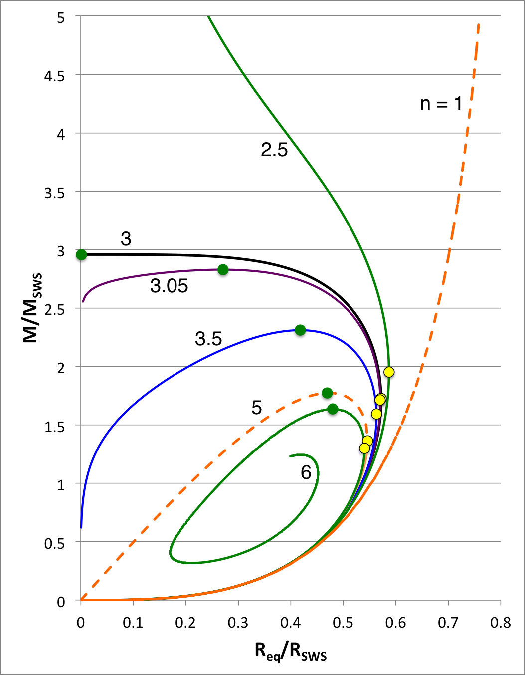
Figure 1: Equilibrium Sequences of Pressure-Truncated Polytropes

We expect the content of this chapter — which examines the relative stability of bipolytropes — to parallel in many ways the content of an accompanying chapter in which we have successfully analyzed the relative stability of pressure-truncated polytopes. Figure 1, shown here on the right, has been copied from a closely related discussion. The curves show the mass-radius relationship for pressure-truncated model sequences having a variety of polytropic indexes, as labeled, over the range <math>1 \le n \le 6</math>. (Another version of this figure includes the isothermal sequence.) On each sequence for which <math>~n \ge 3</math>, the green filled circle identifies the model with the largest mass. We have shown analytically that the oscillation frequency of the fundamental-mode of radial oscillation is precisely zero^† for each one of these maximum-mass models. As a consequence, we know that each green circular marker identifies the point along its associated sequence that separates dynamically stable (larger radii) from dynamically unstable (smaller radii) models.

^†In each case, the fundamental-mode oscillation frequency is precisely zero if, and only if, the adiabatic index governing expansions/contractions is related to the underlying structural polytropic index via the relation, <math>~\gamma_g = (n + 1)/n</math>, and if a constant surface-pressure boundary condition is imposed.

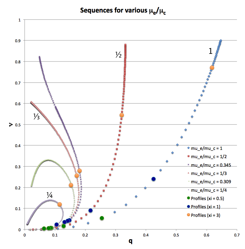
In another accompanying chapter, we have used purely analytic techniques to construct equilibrium sequences of spherically symmetric bipolytropes that have, <math>~(n_c,n_e) = (5,1)</math>. For a given choice of <math>~\mu_e/\mu_c</math> — the ratio of the mean-molecular weight of envelope material to the mean-molecular weight of material in the core — a physically relevant sequence of models can be constructed by steadily increasing the value of the dimensionless radius at the core/envelope interface, <math>~\xi_i</math>, from zero to infinity. Figure 2, which has been copied from this separate chapter, shows how the fractional core mass, <math>\nu \equiv M_\mathrm{core}/M_\mathrm{tot}</math>, varies with the fractional core radius, <math>q \equiv r_\mathrm{core}/R</math>, along sequences having six different values of <math>~\mu_e/\mu_c</math>: 1 (blue diamonds), ½ (red squares), 0.345 (dark purple crosses), ⅓ (pink triangles), 0.309 (light green dashes), and ¼ (purple asterisks). Along each of the model sequences, points marked by solid-colored circles correspond to models whose interface parameter, <math>~\xi_i</math>, has one of three values: 0.5 (green circles), 1 (dark blue circles), or 3 (orange circles).

When modeling bipolytropes, the default expectation is that an increase in <math>\xi_i</math> along a given sequence will correspond to an increase in the relative size — both the radius and the mass — of the core. As Figure 2 illustrates, this expectation is realized along the sequences marked by blue diamonds (<math>~\mu_e/\mu_c = 1</math>) and by red squares (<math>~\mu_e/\mu_c = </math>½). But the behavior is different along the other four illustrated sequences. For sufficiently large <math>~\xi_i</math>, the relative radius of the core begins to decrease. Furthermore, along sequences for which <math>~\mu_e/\mu_c < \tfrac{1}{3}</math>, eventually the fractional mass of the core reaches a maximum and, thereafter, decreases even as the value of <math>~\xi_i</math> continues to increase. (Additional properties of these equilibrium sequences are discussed in yet another accompanying chapter.)

The principal question is: Are these maximum-mass models associated with the onset of dynamical instabilities along bipolytropic sequences?

Planned Approach

Figure 2: Equilibrium Sequences of Bipolytropes with <math>~(n_c,n_e) = (5,1)</math>

Ideally we would like to answer the just-stated "principal question" using purely analytic techniques. But, to date, we have been unable to fully address the relevant issues analytically, even in what would be expected to be the simplest case: bipolytropic models that have <math>~(n_c,n_e) = (0, 0)</math>. Instead, we will streamline the investigation a bit and proceed — at least initially — using a blend of techniques. We will investigate the relative stability of bipolytropic models having <math>~(n_c,n_e) = (5,1) </math> whose equilibrium structures are completely defined analytically; then the eigenvectors describing radial modes of oscillation will be determined, one at a time, by solving the relevant LAWE(s) numerically. We are optimistic that this can be successfully accomplished because we have had experience numerically integrating the LAWE that governs the oscillation of isolated <math>~n = 3</math> polytropes and, separately, the LAWE that governs the oscillation of pressure-truncated isothermal spheres.

A key reference throughout this investigation will be the paper by J. O. Murphy & R. Fiedler (1985b, Proc. Astr. Soc. of Australia, 6, 222). They studied Radial Pulsations and Vibrational Stability of a Sequence of Two Zone Polytropic Stellar Models. Specifically, their underlying equilibrium models were bipolytropes that have <math>~(n_c,n_e) = (1, 5)</math>. In an accompanying chapter, we describe in detail how Murphy & Fiedler obtained these equilibrium bipolytropic structures and detail some of their equilibrium properties.

Here are the steps we initially plan to take:

Governing LAWEs:
- Identify the relevant LAWEs that govern the behavior of radial oscillations in the <math>~n_c = 5</math> core and, separately, in the <math>~n_e = 1</math> envelope. Check these LAWE specifications against the published work of Murphy & Fiedler (1985b).
- Determine the matching conditions that must be satisfied across the core/envelope interface. Be sure to take into account the critical interface jump conditions spelled out by P. Ledoux & Th. Walraven (1958), as we have already discussed in the context of an analysis of radial oscillations in zero-zero bipolytropes.
Determine what surface boundary condition should be imposed on physically relevant LAWE solutions, i.e., on the physically relevant radial-oscillation eigenvectors.
Initial Analysis:
- Choose a maximum-mass model along the bipolytropic sequence that has, for example, <math>~\mu_e/\mu_c = 1/4</math>. Hopefully, we will be able to identify precisely (analytically) where this maximum-mass model lies along the sequence. Yes! Our earlier analysis does provide an analytic prescription of the model that sits at the maximum-mass location along the chosen sequence.
- Solve the relevant eigenvalue problem for this specific model, initially for <math>~(\gamma_c, \gamma_e) = (6/5, 2)</math> and initially for the fundamental mode of oscillation.

Begin Analysis

Relevant LAWEs

The LAWE that is relevant to polytropic spheres may be written as,

	<math>~0 = \frac{d^2x}{d\xi^2} + \biggl[ 4 - (n+1) Q \biggr] \frac{1}{\xi} \cdot \frac{dx}{d\xi} + (n+1) \biggl[ \biggl( \frac{\sigma_c^2}{6\gamma_g } \biggr) \frac{\xi^2}{\theta} - \alpha Q\biggr] \frac{x}{\xi^2} </math>
where: <math>~Q(\xi) \equiv - \frac{d\ln\theta}{d\ln\xi} \, ,</math> <math>~\sigma_c^2 \equiv \frac{3\omega^2}{2\pi G\rho_c} \, ,</math> and, <math>~\alpha \equiv \biggl(3 - \frac{4}{\gamma_\mathrm{g}}\biggr)</math>

Structural Layers With n = 1

The LAWE for n = 1 structures is, then,

<math>~0 = \frac{d^2x}{d\xi^2} + \biggl[ 4 - (n+1) Q \biggr] \frac{1}{\xi} \cdot \frac{dx}{d\xi} + (n+1) \biggl[ \biggl( \frac{\sigma_c^2}{6\gamma_g } \biggr) \frac{\xi^2}{\theta} - \alpha Q\biggr] \frac{x}{\xi^2} </math>

where: <math>~Q(\xi) \equiv - \frac{d\ln\theta}{d\ln\xi} \, ,</math> <math>~\sigma_c^2 \equiv \frac{3\omega^2}{2\pi G\rho_c} \, ,</math> and, <math>~\alpha \equiv \biggl(3 - \frac{4}{\gamma_\mathrm{g}}\biggr)</math>

Structural Layers With n = 5

And for n = 5 structures the LAWE is,

<math>~0 = \frac{d^2x}{d\xi^2} + \biggl[ 4 - (n+1) Q \biggr] \frac{1}{\xi} \cdot \frac{dx}{d\xi} + (n+1) \biggl[ \biggl( \frac{\sigma_c^2}{6\gamma_g } \biggr) \frac{\xi^2}{\theta} - \alpha Q\biggr] \frac{x}{\xi^2} </math>

where: <math>~Q(\xi) \equiv - \frac{d\ln\theta}{d\ln\xi} \, ,</math> <math>~\sigma_c^2 \equiv \frac{3\omega^2}{2\pi G\rho_c} \, ,</math> and, <math>~\alpha \equiv \biggl(3 - \frac{4}{\gamma_\mathrm{g}}\biggr)</math>

User:Tohline/SSC/Stability/BiPolytropes

Contents