Summary for Hadley & Imamura

[Comment by J. E. Tohline on 24 May 2016] This chapter contains a set of technical notes and accompanying discussion that I put together several months ago as I was trying to gain a foundational understanding of the results of a large study of instabilities in self-gravitating tori published by the Imamura & Hadley collaboration. I have come to appreciate that some of the logic and interpretation of published results that are presented, below, has serious flaws. Therefore, anyone reading this should be quite cautious in deciding what subsections provide useful insight. I have written a separate chapter titled, "Characteristics of Unstable Eigenvectors in Self-Gravitating Tori," that contains a much more trustworthy analysis of this very interesting problem.

Material that appears after this point in our presentation is under development and therefore
may contain incorrect mathematical equations and/or physical misinterpretations.
| Go Home |

This MediaWiki-based document is especially provided for Jimmy Imamura and Kathryn Hadley. It summarizes the contents of a much longer set of technical notes that discusses the analysis of nonaxisymmetric distortions in rotating, self-gravitating fluids. The punchline is provided by the animation sequence shown in Figure 2, below.

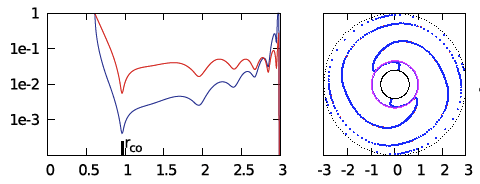
While studying the series of three papers that has recently been published by the Imamura & Hadley collaboration, I was particularly drawn to the pair of plots presented in Figure 6 — and, again, in the top portion of Figure 13 and the top portion of Figure 16 — of HI11. This pair of plots has been reprinted here, without modification, as our Figure 1. The curves delineated by the blue dots in this pair of HI11 plots display (on the left) the shape of the eigenfunction, <math>~f_1(\varpi)</math>, and (on the right) the "constant phase locus," <math>~\phi_1(\varpi)</math>, for an unstable, <math>~m=1</math> mode. In this case, the initial model for the depicted evolution is the equilibrium model from Table 2 of HI11 that has <math>~T/|W| = 0.253</math>; it is a fully self-gravitating torus with polytropic index, <math>~n = 3/2</math>, and a rotation-law profile defined by a "Keplerian" angular velocity profile.

Figure 1

Panel pair extracted^† without modification from the top-most segment of Figure 13, p. 18 of K. Hadley & J. N. Imamura (2011)

"Nonaxisymmetric Instabilities of Self-Gravitating Disks. I Toroids"

Astrophysics and Space Science, 334, 1 - 26 © Springer Science+Business Media B.V.

^†This pair of plots also appears in the top portion of Figure 16 on p. 20 and, by itself, as Figure 6 on p. 12 of K. Hadley & J. N. Imamura (2011).

Radial Eigenfunction

Recognition #1

It occurred to me, first, that the blue curve displayed in the left-hand panel of Figure 1 might be reasonably well approximated by piecing together a pair of arc-hyperbolic-tangent (ATANH) functions. In an effort to demonstrate this, I began by specifying a "midway" radial location, <math>~r_- < r_\mathrm{mid} < r_+ \, ,</math> at which the two ATANH functions meet and at which the density fluctuation is smallest. Then I defined a function of the form,

	<math>~f_\ln(\varpi)</math>	<math>~=</math>	<math>~\tanh^{-1}\biggl[1 - 2 \biggl( \frac{\varpi - r_-}{r_\mathrm{mid}-r_-} \biggr) \biggr]</math>	for	<math>r_- < \varpi < r_\mathrm{mid} \, ;</math>
and
	<math>~f_\ln(\varpi)</math>	<math>~=</math>	<math>~\tanh^{-1}\biggl[1 - 2 \biggl( \frac{\varpi - r_+}{r_\mathrm{mid}-r_+} \biggr) \biggr]</math>	for	<math>r_\mathrm{mid} < \varpi < r_+ \, .</math>

Recognizing that the figure depicting the HI11 eigenfunction is a semi-log plot, it seems clear that the relationship between our constructed function, <math>~f_\ln(\varpi)</math>, and the eigenfunction, <math>~f_1(\varpi)</math>, is,

<math>~f_1(\varpi) = e^{f_\ln(\varpi)} \, .</math>

Recognition #2

Given that, in general, the following mathematical relation holds,

<math>~\ln\biggl( \frac{1+x}{1-x} \biggr)^{1/2} </math>

for

we can write for the innermost region of the toroidal configuration — that is, over the lower radial-coordinate range —

<math>~f_1(\varpi) = e^{f_\ln(\varpi)}</math>

<math>~\biggl( \frac{r_\mathrm{mid} - \varpi}{\varpi - r_-} \biggr)^{1/2} </math>

for

Similarly, we find that, over the upper radial-coordinate range,

<math>~f_1(\varpi) = e^{f_\ln(\varpi)}</math>

<math>~\biggl( \frac{r_\mathrm{mid} - \varpi}{\varpi - r_+} \biggr)^{1/2} </math>

for

<math>r_\mathrm{mid} < \varpi < r_+ \, .</math>

Recognition #3

After a bit more experimentation, we recognized that it is advantageous to replace the square root — that is, the exponent, ½ — with a variable exponent, <math>~p</math>, that can serve as an adjustable fitting parameter; and, in order to facilitate a degree of radial overlap between the two ATANH functions, we introduced different values of <math>~r_\mathrm{mid}</math> on the left and on the right. This led to a two-piece radial eigenfunction of the form,

<math>~f_\mathrm{blue}(\varpi) </math>

<math>~\biggl( \frac{r_\mathrm{blue} - \varpi}{\varpi - r_-} \biggr)^{p} </math>

for

<math>r_- < \varpi < r_\mathrm{blue} </math> … <math>~\biggl[ f_\mathrm{blue}(\varpi) = 0</math> otherwise<math>~\biggr]</math>,

and,

<math>~f_\mathrm{green}(\varpi) </math>

<math>~\biggl( \frac{r_\mathrm{green} - \varpi}{\varpi - r_+} \biggr)^{p} </math>

for

<math>r_\mathrm{green} < \varpi < r_+ </math> … <math>~\biggl[ f_\mathrm{green}(\varpi) = 0</math> otherwise<math>~\biggr]</math>,

where, <math>~r_\mathrm{mid}|_\mathrm{green} \le r_\mathrm{mid}|_\mathrm{blue}</math>.

Summary

The expression that we are currently using for the radial eigenfunction is a sum of these two pieces, that is,

<math>~f_1(\varpi)</math>

<math>~f_\mathrm{green}(\varpi) + f_\mathrm{blue}(\varpi) \, . </math>

For later use, we define from this function the minimum and maximum values,

<math>~[f_\ln]_\mathrm{min} \equiv \mathrm{min}[\ln(f_1)]</math>

and

<math>~[f_\ln]_\mathrm{max} \equiv \mathrm{max}[\ln(f_1)] \, .</math>

Constant Phase Loci

As is explained in our accompanying detailed technical notes — see, also another improvement — we have settled on the following prescription for the phase function, <math>~\phi_m(\varpi)</math>:

<math>~\pm \tan^{-1}[\aleph_m \cdot D_{1/2}(\varpi)] \, .</math>

where,

<math>~D_{1/2}(\varpi)</math>

<math>~\equiv</math>

<math>~\biggl[ \frac{f_\ln(\varpi) - [f_\ln]_\mathrm{min}}{[f_\ln]_\mathrm{max} - [f_\ln]_\mathrm{min}} \biggr]^{1/2} \, ,</math>

<math>~\aleph_m</math> is a (perhaps, mode-dependent) constant to be specified, and,

<math>~f_\ln(\varpi)</math>

<math>~\equiv</math>

<math>~\ln[ f_1(\varpi)] \, .</math>

Put It Together

Figure 2a contains an animation sequence that is intended to illustrate that our empirically constructed radial eigenfunction and accompanying polar-coordinate plots of "constant phase loci" closely resemble the radial eigenfunctions and constant phase loci that have been displayed in HI11's Figure 16 (a portion of which is redisplayed, here, as Figure 2b). Each frame of the Figure 2a animation, contains (on the left) a semi-log plot of <math>~f_1(\varpi)</math> versus <math>~\varpi</math> and (on the right) the corresponding constant phase loci that are generated for <math>~\phi_1</math> (top), <math>~\phi_2</math> (middle), and <math>~\phi_3</math> (bottom), when the natural log of the same function, <math>~f_\ln = \ln[f_1(\varpi)]</math>, is plugged into our empirically derived function, <math>~D_{1/2}</math>. In a separate chapter we demonstrate in more detail how each frame of this animation sequence was constructed. As displayed in Figure 2a, <math>~r_\mathrm{green}</math> is the only parameter that is varied from frame to frame of the animation (the seven specified values are listed in a column to the left of the animation); all of the other empirical model parameters — <math>~r_\mathrm{blue}</math>, <math>~p</math>, and <math>~\aleph_m</math> — are held fixed, along with specifications of the inner and outer edges of the torus, <math>~r_-</math> and <math>~r_+</math>.

Figure 2: Radial and Azimuthal Eigenfunction Comparison

(a) Our Empirically Constructed Function

(b) Extracted from Figure 16 of HI11

Specified <math>~r_\mathrm{green}</math>	Resulting <math>~r_\mathrm{min}</math>
1.10324	1.103
1.05929	1.077
1.01534	1.059
0.97139	1.042
0.88349	1.020
0.75164	0.998
0.61979	0.976

Notice that, by simply varying the value of <math>~r_\mathrm{green}</math>, our semi-log plot of <math>~f_1</math> versus <math>~\varpi</math> sweeps through shapes that qualitatively match the three radial eigenfunctions (see Figure 2b) that arose in the HI11 investigation. At the largest value, <math>~r_\mathrm{green} = 1.10324</math> (1^st frame of the animation loop), the minimum of the radial eigenfunction is sharply defined and sits at <math>~r_\mathrm{min} = 1.103</math>, as labeled in the animation; the <math>~f_1(\varpi)</math> eigenfunction displayed in this particular frame closely resembles the radial eigenfunction shown at the top of the HI11 figure and, simultaneously, the <math>~m=1</math> "constant phase locus" plot that appears in the same frame of the animation closely resembles the <math>~m=1</math> constant phase locus that is displayed at the top of the HI11 figure. When we set <math>~r_\mathrm{green} = 1.05929</math> (2^nd frame of the animation), the minimum of the radial eigenfunction is still well-defined and sits at <math>~r_\mathrm{min} = 1.077</math>, as labeled in the animation. The <math>~f_1(\varpi)</math> eigenfunction displayed in this 2^nd frame closely resembles the radial eigenfunction shown in the middle panel of the HI11 figure and, simultaneously, the <math>~m=2</math> "constant phase locus" plot that appears in this 2^nd frame of the animation closely resembles the <math>~m=2</math> constant phase locus that is displayed at the middle of the HI11 figure.

Additional Comments

I was delighted to be able to find a single function, such as <math>f_\ln = \ln[f_1(\varpi)]</math>, that can pretty faithfully represent, not just one, but a set of HI11's observed eigenfunctions by simply adjusting one parameter, <math>~f_\mathrm{green}</math>. I was quite happy with this finding and, originally, had no expectation that the function, <math>~f_\ln</math>, would in any way relate to the functional behavior of the corresponding "constant phase loci." After all, it seemed to me that, in general, one should expect that an eigenvector's "amplitude" and "phase" functions will be totally independent of one another.
I was extraordinarily pleased — and stunned! — to find that the same function, <math>~f_\ln</math>, also could be used to provide a reasonably faithful representation of the phase function, <math>~\phi(\varpi)</math>.
In retrospect, it seems clear that the pairs of "amplitude" and "phase" plots published by the Imamura & Hadley collaboration for various unstable eigenmodes do exhibit a strong degree of interdependence:
1. The radial location, <math>~r_\mathrm{min}</math>, at which the "amplitude" plot exhibits a minimum (identified, for example, by the red, vertical, dashed line in our Figure 2a animation) also appears to be the radial location at which the "phase" plot exhibits a rapid phase swing (identified by the red, dashed circle in our Figure 2a animation).
2. The degree to which a given "constant phase locus" exhibits a rapid phase swing appears to correlate with the steepness of the <math>~f_\ln(\varpi)</math> function. If the "amplitude" plot exhibits a sharp, well-defined minimum, then the "phase" plot exhibits a sharp phase swing; conversely, if the "amplitude" plot is rather smooth and featureless, then the "phase" plot exhibits milder phase swings.
3. Then, of course, there are examples such as the one displayed here, on the right, taken from Figure 4 in Paper 2 (Hadley et al. 2014) in which the number of times the "constant phase locus" plot swings through a full <math>~2\pi</math> radians correlates with the number of local minima exhibited by the corresponding "amplitude" plot.
It has occurred to me that each local minimum in an "amplitude" plot may be representing a radial node of the underlying (Lagrangian) radial displacement function, <math>~\delta r/r</math>. Related thoughts:
1. The density fluctuation may flip its sign — going from a positive to a negative fluctuation, for example — each time our traditional "amplitude" plot passes through a local minimum, in which case our traditional "amplitude" plot is really presenting (in some sense) the absolute value of the density fluctuation.
2. This idea is easier to swallow when we recognize that our traditional "amplitude" plot is a semi-log plot; on a linear scale, the minima indicate that the function is dropping close to zero, so it is not unreasonable to propose that the fluctuation is passing through zero at these radial locations.
3. This would also help explain why, during my empirical construction of each "constant phase locus" plot, I presently have to manually flip the sign on the phase function, <math>~\phi_1(\varpi)</math>, when crossing the radial location of a local minimum, <math>~r_\mathrm{min}</math>.

Material that appears after this point in our presentation is under development and therefore
may contain incorrect mathematical equations and/or physical misinterpretations.
| Go Home |

Analytic Analysis of Zero-Mass Papaloizou-Pringle Tori

Here we present a summary of a much more detailed, accompanying derivation.

Generic Formulation

As is explicitly defined in Figure 1 of our accompanying detailed notes, we have chosen to represent the spatial structure of an eigenfunction in the equatorial-plane of toroidal-like configurations via the expression,

<math>~\biggl[ \frac{\delta\rho}{\rho_0}\biggr]_\mathrm{spatial} </math>

<math>~\biggl\{ f_m(\varpi)e^{-im\phi} \biggr\} \, .</math>

In general, we should assume that the function that delineates the radial dependence of the eigenfunction has both a real and an imaginary component, that is, we should assume that,

<math>~f_m(\varpi)</math>

<math>~\mathcal{A}(\varpi) + i\mathcal{B}(\varpi) \, ,</math>

in which case the square of the modulus of the function is,

<math>~|f_m|^2 \equiv f_m \cdot f^*_m </math>

<math>~\mathcal{A}^2 + \mathcal{B}^2 \, .</math>

We can rewrite this complex function in the form,

<math>~f_m(\varpi)</math>

<math>~|f_m|e^{-i[\alpha(\varpi) + \pi/2]} \, ,</math>

if the angle, <math>~\alpha(\varpi)</math> is defined such that,

<math>~\sin\alpha = \frac{\mathcal{A}}{\sqrt{\mathcal{A}^2 + \mathcal{B}^2}}</math>	and	<math>~\cos\alpha = \frac{\mathcal{B}}{\sqrt{\mathcal{A}^2 + \mathcal{B}^2}}</math>
<math>~\Rightarrow ~~~~ \alpha</math>	<math>~\equiv</math>	<math>~\tan^{-1}\biggl(\frac{\mathcal{A}}{\mathcal{B}}\biggr) = \tan^{-1}\biggl[ \frac{\mathrm{Re}(f_m)}{\mathrm{Im}(f_m)} \biggr] \, .</math>

Hence, the spatial structure of the eigenfunction can be rewritten as,

<math>~\biggl[ \frac{\delta\rho}{\rho_0}\biggr]_\mathrm{spatial} </math>

<math>~|f_m(\varpi)|e^{-i[\alpha(\varpi) + \pi/2+ m\phi]} \, . </math>

From this representation we can see that, at each radial location, <math>~\varpi</math>, the phase angle(s) at which the fractional perturbation exhibits its maximum amplitude, <math>~|f_m|</math>, is identified by setting the exponent of the exponential to zero. That is,

<math>~\phi = \phi_\mathrm{max}(\varpi)</math>

<math>~\equiv</math>

<math>~-\frac{1}{m}\biggl[\alpha(\varpi) +\frac{\pi}{2}\biggr] = -\frac{1}{m}\biggl\{ \tan^{-1}\biggl[ \frac{\mathrm{Re}(f_m)}{\mathrm{Im}(f_m)} \biggr] +\frac{\pi}{2} \biggr\} \, .</math>

An equatorial-plane plot of <math>~\phi_\mathrm{max}(\varpi)</math> should produce the "constant phase locus" referenced, for example, in recent papers from the Imamura & Hadley collaboration.

It should be noted that the leading (negative) sign that appears on the right-hand side of this expression for <math>~\phi_\mathrm{max}</math> is rather arbitrary, as is the additional <math>~\pi/2</math> phase shift that appears in that right-hand side expression. Henceforth, for simplicity, we will omit both and use, instead,

<math>~m\phi_\mathrm{max}(\varpi)</math>

<math>~\equiv</math>

<math>~\tan^{-1}\biggl[ \frac{\mathrm{Re}(f_m)}{\mathrm{Im}(f_m)} \biggr] \, ,</math>

unless and until the sign and/or a global phase shift is needed to adjust the orientation of a "constant phase locus" plot to facilitate comparison with published figures.

Blaes (1985)

His Derived Eigenfunction

Via an analytic perturbation analysis, Blaes (1985) shows that, in slender PP tori with uniform specific angular momentum, the spatial structure of unstable modes can be expressed as,

<math>~\frac{W(\eta,\theta)}{W_0} -1</math>

<math>~\biggl\{ f_m(\eta,\theta)e^{-i[m\phi + k\theta]} \biggr\} \, ,</math>

where (see his equation 1.10),

<math>~f_m(\eta,\theta)</math>

<math> ~\beta^2 m^2 \biggl[ 2\eta^2 \cos^2\theta - \frac{3\eta^2}{4(n+1)} - \frac{(4n+1)}{4(n+1)^2} \pm 4i\biggl(\frac{3}{2n+2}\biggr)^{1/2} \eta\cos\theta\biggr] + \mathcal{O}(\beta^3) \, . </math>

In this expression, <math>~n</math> is the polytropic index, and <math>~\beta</math> is a dimensionless parameter that specifies the relative thickness of the torus; specifically, in terms of the ratio of the inner-to-outer edge of the torus, <math>~r_-/r_+</math>,

<math>~\beta \equiv \frac{1- r_-/r_+}{1+ r_-/r_+} \, .</math>

Notice that this eigenfunction derived by Blaes (1985) describes a spatial perturbation that is not confined to the equatorial plane of the torus. The parameter pair, <math>~(\eta,\theta)</math>, defines a two-dimensional, polar coordinate system in a plane lying perpendicular to the equatorial plane that contains the torus's (nearly circular) cross-section: <math>~\eta</math> is a dimensionless radial coordinate measuring distance from the center of the cross-section — <math>~\eta = 0</math> at the center of the cross-section and <math>~\eta = 1</math> at the surface of the torus; and <math>~\theta</math> is the polar-coordinate oriented such that <math>~\theta = 0</math> points toward the "inner" edge of the torus, <math>~\theta = \pi/2</math> points vertically, straight "up," and <math>~\theta = \pi</math> points toward the "outer" edge of the torus.

Paralleling the generic formulation that has just been discussed, this is a complex function having, to lowest order, the following real and imaginary parts:

<math>~\mathcal{A}_\mathrm{Blaes}(\eta,\theta)</math>	<math>~=</math>	<math>~(\beta m)^2\biggl[ 2\eta^2 \cos^2\theta - \frac{3\eta^2}{4(n+1)} - \frac{(4n+1)}{4(n+1)^2} \biggr] </math>
	<math>~=</math>	<math>~\frac{ (\beta m)^2}{4(n+1)^2}\biggl\{ ~[8(n+1)\cos^2\theta - 3]\eta^2 (n+1) - (4n+1) \biggr\} \, ; </math>
<math>~\mathcal{B}_\mathrm{Blaes}(\eta,\theta)</math>	<math>~=</math>	<math>~ 4(\beta m)^2\biggl(\frac{3}{2n+2}\biggr)^{1/2} \eta\cos\theta </math>
	<math>~=</math>	<math>~\frac{(\beta m)^2}{4(n+1)^2}\biggl[2^7\cdot 3(n+1)^3 \eta^2\cos^2\theta \biggr]^{1/2}\, . </math>

We should therefore find that the amplitude (modulus) of the perturbation is,

<math>~\biggl|\frac{W}{W_0} -1\biggr|</math>

<math>~\sqrt{\mathcal{A}_\mathrm{Blaes}^2+ \mathcal{B}_\mathrm{Blaes}^2} \, ;</math>

and the associated "constant phase locus" should be identified by the function,

<math>~m\phi_\mathrm{max}(\eta,\theta)</math>

<math>~ \tan^{-1}\biggl[ \frac{\mathcal{A}_\mathrm{Blaes}}{\mathcal{B}_\mathrm{Blaes}} \biggr] - k\theta \, .</math>

Nice Features

After summarizing, above, our efforts to develop (by empirical techniques) mathematical expressions that qualitatively match the shape of unstable eigenfunctions in toroidal configurations, we put together a subsection titled, "Additional Comments," to highlight ways in which the empirical fits were successful and ways in which they fell short of expectations. Here, following our presentation of Blaes's (1985) analytically derived eigenfunction for slim PP tori, we highlight elements of his (physically justified) eigenfunction that explain the origin of many features that were highlighted, above.

The "amplitude" plot and a plot of the "constant phase locus" should, indeed, appear to be interdependent because they both depend on the functional forms of <math>~\mathcal{A}</math> and <math>~\mathcal{B}</math>; in the end, however, the two plots are formally independent of one another.
The square of the modulus — that is, the "amplitude" plot — should always be the sum of two independent functions, both of which are intrinsically positive.
If either <math>~\mathcal{A}</math> or <math>~\mathcal{B}</math> is defined by a function that crosses zero (perhaps multiple times) with a naturally continuous derivative, that function can quite naturally give rise to a "log-amplitude" plot that shoots toward minus infinity and exhibits a discontinuous derivative after the function is squared to become a piece of the "modulus" expression.
It is now easy to understand why the earlier "empirically derived" constant phase loci were phrased in terms of the arctangent function.
Each "constant phase locus" plot should naturally be composed of two (smoothly joined) pieces: One defined over the inner portion of the torus — <math>~\eta</math> goes from zero to 1 while <math>~\theta = 0</math>; and one defined over the outer portion of the torus — <math>~\eta</math> goes from zero to 1 while <math>~\theta = \pi</math>.
Because (at least for slim PP-tori) the ratio, <math>~\mathcal{A}/\mathcal{B}</math> contains an overall factor that is an odd power of <math>~\cos\theta</math>, the argument of the arctangent function will automatically flip signs as we move from the "inner" region of the torus to the "outer" region of the torus.
We now appreciate that a plot of "constant phase locus" is smooth across the mid-point (across the cross-sectional center) of the torus because the definition of <math>~\phi_\mathrm{max}</math> naturally contains a phase shift of <math>~k\theta</math>.

Movie

Figure 3 displays, for various values of the polytropic index, <math>~0.0 \le n\le 5.0</math>, the radial structure of the Blaes85 <math>~m=2</math> eigenfunction for a slim PP-torus having <math>~\beta = 0.18</math>. More specifically, for each frame of the animation, the figure displays as a function of the dimensionless radial coordinate, <math>~x</math>, (left panel) the behavior of

Left: <math>~\sqrt{\mathcal{A}_\mathrm{Blaes}^2 + \mathcal{B}_\mathrm{Blaes}^2}</math>

on a semi-log plot; and (right panel) the "constant phase locus,"

Right: <math>~\frac{1}{2} \tan^{-1} \biggl[ \frac{\mathcal{A}_\mathrm{Blaes}}{\mathcal{B}_\mathrm{Blaes}} \biggr] - \theta \, .</math>

Figure 3: The Blaes85 Analytic Eigenfunction

CAPTION: Radial dependence of the (left) amplitude and (right) "constant phase locus" of the Blaes85 analytic eigenfunction, for various values of the polytropic Index, <math>~n</math>, as indicated in the bottom-right corner of the left panel.

Comparisons

For n = 3 Configurations

Following §1.3 of Blaes85, let's specifically consider the case of slim PP-tori that have a polytropic index, <math>~n=3</math>. In this case, we have,

<math>~\mathcal{A}_\mathrm{Blaes}(\eta,\theta)</math>	<math>~=</math>	<math>~\frac{ (\beta m)^2}{2^6}\biggl[a_3(\eta,\theta)\biggr] \, , </math>
<math>~\mathcal{B}_\mathrm{Blaes}(\eta,\theta)</math>	<math>~=</math>	<math>~\frac{(\beta m)^2}{2^6}\biggl[b_3(\eta,\theta)\biggr] \, , </math>

where,

<math>~a_3(\eta,\theta)</math>	<math>~\equiv</math>	<math>~\biggl\{ ~[8(n+1)\cos^2\theta - 3]\eta^2 (n+1) - (4n+1) \biggr\}_{n=3} </math>
	<math>~=</math>	<math>~ ~2^2[2^5\cos^2\theta - 3]\eta^2 - 13 \, , </math>
<math>~b_3(\eta,\theta)</math>	<math>~\equiv</math>	<math>~\biggl\{ [2^7\cdot 3(n+1)^3 \eta^2\cos^2\theta ]^{1/2} \biggr\}_{n=3} </math>
	<math>~=</math>	<math>~[2^{13}\cdot 3\eta^2\cos^2\theta ]^{1/2}\, . </math>

Now, rather than examining the structural behavior of the amplitude and phase of the function, <math>~[W/W_0 -1]</math>, as we have done, above, Blaes evaluated the amplitude (only) of the function,

<math>~\frac{W}{W_0} = 1 + \mathcal{A}_\mathrm{Blaes}(\eta,\theta) + i \mathcal{B}_\mathrm{Blaes}(\eta,\theta) \, .</math>

For the specific case of <math>~n=3</math>, the square of the amplitude of this function is,

<math>~\biggl\|\frac{W}{W_0} \biggr\|_{n=3}^2</math>	<math>~=</math>	<math>~\biggl\{ 1 + \frac{ (\beta m)^2}{2^6}\biggl[a_3(\eta,\theta)\biggr] \biggr\}^2 + \biggl\{ \frac{(\beta m)^2}{2^6}\biggl[b_3(\eta,\theta)\biggr] \biggr\}^2 </math>
	<math>~=</math>	<math>~1 + \frac{ (\beta m)^2a_3}{2^5} + \frac{ (\beta m)^4 }{2^{12}} (a_3^2 + b_3^2) </math>
	<math>~=</math>	<math>~1 + \frac{ (\beta m)^2}{2^5} \biggl\{ 2^2[2^5\cos^2\theta - 3]\eta^2 - 13\biggr\} + \mathcal{O}[(\beta m)^4] \, . </math>

Therefore, to lowest order in the "slimness" parameter, <math>~\beta</math>,

<math>~\biggl|\frac{W}{W_0} \biggr|_{n=3}</math>

<math>~\approx</math>

<math>~1 + \frac{ (\beta m)^2}{2^6} \biggl\{ 2^2[2^5\cos^2\theta - 3]\eta^2 - 13\biggr\} \, . </math>

This (almost exactly) matches the amplitude expression derived by Blaes (1985) and evaluated for the specific case of <math>~\beta = (101)^{-1/2}</math> — the relevant equation (1.12) from Blaes85 is digitally reproduced in the table that follows.

Equation (1.12) extracted without modification from p. 556 of Blaes (1985)

"Oscillations of Slender Tori"

Our expression differs from the one published in Blaes85 in one detail: In Blaes85, the pre-factor of the second term inside the curly braces is, evidently, <math>~(\beta m)^2/2^5</math>, which is a factor of two larger than the corresponding pre-factor found in our expression. In our attempt to re-derive the Blaes85 expression (1.12), this extra factor of two disappears when we take the square-root of both sides to obtain the modulus, rather than the square of the modulus. Hopefully further reflection will resolve this discrepancy between our approximate expression for <math>~|W/W_0|_{n=3}</math> and the analogous one presented in Blaes85.

For n = 0 Configurations

As we have discussed elsewhere, Goldreich, Goodman & Narayan (1986, MNRAS, 221, 339) — hereafter, GGN86 — also used analytic techniques to analyze the properties of unstable, nonaxisymmetric eigenmodes in Papaloizou-Pringle tori. They restricted their discussion to slim, incompressible tori, so in order to assess the overlap between the GGN86 and Blaes85 works, we will set <math>~n=0</math> in the general expressions presented in Blaes85.

<math>~\mathcal{A}_\mathrm{Blaes}(\eta,\theta)</math>	<math>~=</math>	<math>~\frac{ (\beta m)^2}{2^2}\biggl[a_0(\eta,\theta)\biggr] \, , </math>
<math>~\mathcal{B}_\mathrm{Blaes}(\eta,\theta)</math>	<math>~=</math>	<math>~\frac{(\beta m)^2}{2^2}\biggl[b_0(\eta,\theta)\biggr] \, , </math>

where,

<math>~a_0(\eta,\theta)</math>	<math>~\equiv</math>	<math>~\biggl\{ ~[8(n+1)\cos^2\theta - 3]\eta^2 (n+1) - (4n+1) \biggr\}_{n=0} </math>
	<math>~=</math>	<math>~ ~[8\cos^2\theta - 3]\eta^2 - 1 \, , </math>
<math>~b_0(\eta,\theta)</math>	<math>~\equiv</math>	<math>~\biggl\{ [2^7\cdot 3(n+1)^3 \eta^2\cos^2\theta ]^{1/2} \biggr\}_{n=0} </math>
	<math>~=</math>	<math>~2^3 (2\cdot 3)^{1/2} \eta \cos\theta \, . </math>

From the Blaes85 analysis, then, we conclude that the unstable eigenfunction for slim, incompressible PP-tori is,

<math>~\biggl[ \frac{W}{W_0}\biggr]_{n=0}</math>	<math>~=</math>	<math>~1 + \frac{ (\beta m)^2}{2^2}\biggl[(8\cos^2\theta - 3)\eta^2 - 1\biggr] + i \frac{ (\beta m)^2}{2^2}\biggl[ 2^3 (2\cdot 3)^{1/2} \eta \cos\theta \biggr] </math>
	<math>~=</math>	<math>~\biggl[1 - \tfrac{1}{4}(\beta m)^2\biggr] + (\beta m)^2 \biggl[\biggl(2\cos^2\theta - \frac{3}{4}\biggr)\eta^2 \biggr] + 4i (\beta m)^2\biggl[ \biggl(\frac{3}{2}\biggr)^{1/2} \eta \cos\theta \biggr] \, . </math>

This should be compared with equation (5.16) of GGN86, which is "the lowest order [complex] expression for the [perturbed] velocity potential," namely,

<math>~\psi </math>	<math>~=</math>	<math>~1+\tfrac{1}{4} k^2(5x^2 - 3z^2) \mp 4i\biggl(\frac{3}{2}\biggr)^{1/2} k x \beta_\mathrm{GGN} </math>
	<math>~=</math>	<math>~1+m^2 \beta^2_\mathrm{Blaes}\biggl[2\eta^2\cos^2\theta - \frac{3\eta^2}{4}\biggr] \mp 4i \biggl(\frac{3}{2}\biggr)^{1/2} m^2\beta^2_\mathrm{Blaes} \eta\cos\theta \, ,</math>

where the last expression results from our mapping of the GGN86 terminology to the Blaes85 terminology. The two derived expressions match in every detail, except one: The constant term, <math>~\tfrac{1}{4}(\beta m)^2</math>, that is subtracted from unity on the right-hand side of the Blaes85 function is missing from the function derived by GGN86. Hopefully, additional study of this problem will rectify this apparent difference between the two published analyses.

For n = 3/2 Configurations

The Imamura & Hadley collaboration examined instabilities that develop in tori having a variety of polytropic indexes, but their focus was often on <math>~n=3/2</math> configurations. It is useful, therefore, to evaluate the Blaes85 eigenfunction for this set of models. In this case,

<math>~\mathcal{A}_\mathrm{Blaes}(\eta,\theta)</math>	<math>~=</math>	<math>~\frac{ (\beta m)^2}{5^2}\biggl[a_{3/2}(\eta,\theta)\biggr] \, , </math>
<math>~\mathcal{B}_\mathrm{Blaes}(\eta,\theta)</math>	<math>~=</math>	<math>~\frac{(\beta m)^2}{5^2}\biggl[b_{3/2}(\eta,\theta)\biggr] \, , </math>

where,

<math>~a_{3/2}(\eta,\theta)</math>	<math>~\equiv</math>	<math>~\biggl\{ ~[8(n+1)\cos^2\theta - 3]\eta^2 (n+1) - (4n+1) \biggr\}_{n=3/2} </math>
	<math>~=</math>	<math>~ ~\frac{5}{2}[20\cos^2\theta - 3]\eta^2 - 7 \, , </math>
<math>~b_{3/2}(\eta,\theta)</math>	<math>~\equiv</math>	<math>~\biggl\{ [2^7\cdot 3(n+1)^3 \eta^2\cos^2\theta ]^{1/2} \biggr\}_{n=3/2} </math>
	<math>~=</math>	<math>~[2^{4}\cdot 3\cdot 5^3\eta^2\cos^2\theta ]^{1/2}\, . </math>

Hence, the "constant phase locus" should be identified by the function,

<math>~m\phi_\mathrm{max}(\eta,\theta)</math>	<math>~=</math>	<math>~ \tan^{-1}\biggl\{ \frac{a_{3/2}(\eta,\theta) }{ b_{3/2}(\eta,\theta) } \biggr\} - k\theta </math>
	<math>~=</math>	<math>~ \tan^{-1}\biggl\{ \frac{- 7 + \frac{5}{2}[20\cos^2\theta - 3]\eta^2 }{ 20\cdot (3\cdot 5)^{1/2}\eta \cos\theta } \biggr\} - k\theta </math>
	<math>~=</math>	<math>~ \tan^{-1}\biggl\{ \frac{- 14 + 5[20\cos^2\theta - 3]\eta^2 }{ 40\cdot (3\cdot 5)^{1/2}\eta \cos\theta } \biggr\} - k\theta \, , </math>

and the square of the (unity-adjusted) amplitude is,

<math>~\biggl\|\frac{W}{W_0} - 1 \biggr\|^2</math>	<math>~=</math>	<math>~\frac{ (\beta m)^4 }{5^4} \biggl[ a_{3/2}^2 + b_{3/2}^2 \biggr] </math>
	<math>~=</math>	<math>~ \frac{ (\beta m)^4 }{5^4} \biggl\{ \biggl[\frac{5}{2} (20\cos^2\theta - 3)\eta^2 - 7\biggr]^2 + \biggl[ 2^{4}\cdot 3\cdot 5^3\eta^2\cos^2\theta \biggr] \biggr\} </math>
	<math>~=</math>	<math>~ \frac{ (\beta m)^4 }{5^4} \biggl\{ \biggl[\frac{5}{2} (20\cos^2\theta - 3)\eta^2\biggr]^2 -14 \biggl[\frac{5}{2} (20\cos^2\theta - 3)\eta^2 \biggr] + \biggl[- 7\biggr]^2 + 2^{4}\cdot 3\cdot 5^3\eta^2\cos^2\theta \biggr\} </math>
	<math>~=</math>	<math>~ \frac{ (\beta m)^4 }{5^4} \biggl\{ \frac{5^2}{2^2} (20\cos^2\theta - 3)^2\eta^4 -35 (20\cos^2\theta - 3)\eta^2 + 49 + 6000\eta^2\cos^2\theta \biggr\} </math>
	<math>~=</math>	<math>~ \frac{ (\beta m)^4 }{5^4} \biggl\{49 + [105 + 5300\cos^2\theta ]\eta^2 + \frac{5^2}{2^2} (20\cos^2\theta - 3)^2\eta^4\biggr\} \, . </math>

Let's compare the amplitude and phase diagrams that result from the Blaes85 analytic model with results from the model "P4" evolution reported in Hadley et al. (2014), that is, from Paper II in the Imamura & Hadley collaboration. Setting <math>~n = 3/2</math> and, because this comparison is restricted to the equatorial plane, setting <math>~\theta = 0</math> (inner region of torus) or <math>~\theta = \pi</math> (outer region of torus), we have from Blaes85,

<math>~\mathcal{A}(\eta)</math>	<math>~=</math>	<math> ~\biggl(\frac{17}{10}\biggr)\eta^2 - \frac{7}{25} \, ; </math>
<math>~\mathcal{B}(\eta)</math>	<math>~=</math>	<math>~\pm \biggl(\frac{2^4\cdot 3}{5}\biggr)^{1/2} \eta \, . </math>

Figure 3 presents a plot (left panel) of <math>~\tfrac{1}{4}\mathcal{A}</math> versus <math>~x</math> (salmon-colored markers) and <math>~\tfrac{1}{4}\mathcal{B}</math> versus <math>~x</math> (green markers) for a PP-torus with <math>~\beta = 0.176</math>. This torus has the same aspect ratio as the model named "P4" in Paper II: It has an inner edge at <math>~x_- = 0.85</math>, outer edge at <math>~x_+ = 1.21</math>, and cross-sectional "center" at <math>~x_0 = 1</math>. (For equilibrium model characteristics, also see Table 4 in our accompanying detailed discussion). Via a semi-log plot, the right panel of Figure 3 displays the behavior of <math>~(\tfrac{1}{4}\mathcal{A})^2</math> and <math>~(\tfrac{1}{4}\mathcal{B})^2</math> as a function of <math>~x</math>.

Figure 3: Real (A) and Imaginary (B) Components of the Blaes85 Analytic Eigenfunction

Note that, although the function, <math>~\mathcal{B}(\eta)</math>, is linear in <math>~\eta</math>, the green curve in the left panel of Figure 3 is slightly curved. This is because the horizontal axis (in both panels) is the coordinate, <math>~x</math>, rather than <math>~\eta</math>. The conversion from <math>~\eta</math> to <math>~x</math> is provided by the root of a cubic equation, as discussed separately.

The panel on the right in Figure 3 explains in a qualitative sense how sharp features — in particular, steep valleys — can arise in the "amplitude" plots of simulations that study the nonlinear growth of unstable, nonaxisymmetric eigenmodes in tori. A sharp feature can arise when either the real or the imaginary component of the eigenmode crosses zero (and thereby changes sign). In the analytic eigenfunction expression derived by Blaes (1985), the radial dependence of the imaginary component is defined by a linear function, and it displays a single sharp feature; the radial dependence of the real component is defined by a quadratic function, and it displays a pair of sharp features. It seems clear that, depending on the relative overall amplitude of the real and imaginary parts, the combined amplitude could display a single sharp feature, a pair of sharp features, or a milder curve with no particularly sharp features. It is this third option that results from the specific case presented to us by the Blaes85 eigenfunction. As is shown by the blue curve in the middle-left-hand panel of Figure 4, the Blaes85 modulus — <math>~\tfrac{1}{4}\sqrt{\mathcal{A}^2 + \mathcal{B}^2}</math> — presents a curve with no particularly sharp features.

Figure 4: Comparison

Figure 4 displays (left) the radial dependence of the "amplitude" and (right) the radial dependence of the "constant phase locus" for the unstable modes of three models with similar — although not identical — initial equilibrium structures: (Top row) The model with a star-to-disk mass ratio of 100 labeled "P4" in Paper II of the Imamura & Hadley collaboration; (Middle row) The massless model analyzed analytically by Blaes (1985) and described herein; and (Bottom row) An unpublished model from the Imamura & Hadley collaboration (private communication) with a similar aspect ratio but a star-to-disk mass ratio of 1000.

Various Thoughts

In the Blaes85 model, the "constant phase locus" swings through a total angle of,

<math>~m\Delta</math>

<math>~=</math>

<math>~2\tan^{-1}\biggl[ \frac{\mathcal{A}}{\mathcal{B}} \biggr]_{\eta=1} + \pi \, .</math>

For example, in the model displayed, above, <math>~[\mathcal{A}/\mathcal{B}]_{\eta=1} = 0.4583</math>. Hence, <math>~2\Delta = 4.001</math> radians.
We need to resolve the apparent discrepancy between the value of the leading constant that appears in the GGN86 eigenfunction versus the one that is found in the Blaes85 eigenfunction (when evaluated for <math>~n=0</math>). Graphically, the Blaes85 amplitude function appears to make more sense, but a physically based explanation needs to be identified.
The amplitude and phase functions obtained from the Blaes85 work appear to match — qualitatively, if not quantitatively — the amplitude and phase functions published by the Imamura & Hadley collaboration if we subtract the leading "unity" constant from the Blaes85 expression for <math>~W/W_0</math>. On the other hand, when Blaes refers to the modulus of the amplitude, he includes this leading "unity" constant in evaluating the "real" component of his expression. I do not yet fully understand why both ways of viewing the eigenfunction's amplitude — that is, both with and without including the unity term — can be physically relevant.
As a small extension of the Blaes85 analysis, we should determine what the eigenfunction is for the density perturbation, rather than for the "enthalpy" perturbation, and see how well it matches the blue amplitude and phase curves published by Hadley et al.

User:Tohline/Appendix/Ramblings/To Hadley and Imamura

Contents

Summary for Hadley & Imamura

Radial Eigenfunction

Recognition #1

Recognition #2

Recognition #3

Summary

Constant Phase Loci

Put It Together

Additional Comments

Analytic Analysis of Zero-Mass Papaloizou-Pringle Tori

Generic Formulation

Blaes (1985)

His Derived Eigenfunction

Nice Features

Movie

Comparisons

For n = 3 Configurations

For n = 0 Configurations

For n = 3/2 Configurations

Various Thoughts

See Also

Navigation menu

Search