Cmop
NSF Site Visit
In order to get everything done for the upcoming NSF site visit, I have created this page to share both temporary and complete results as well as to hold discussions on visualization methods being used, why they are employed, and how to better depict data for the scientists in Oregon. Below are links to images and animations showing the current state of visualization of the curvilinear grid simulation sent to me by Yvette.
Images
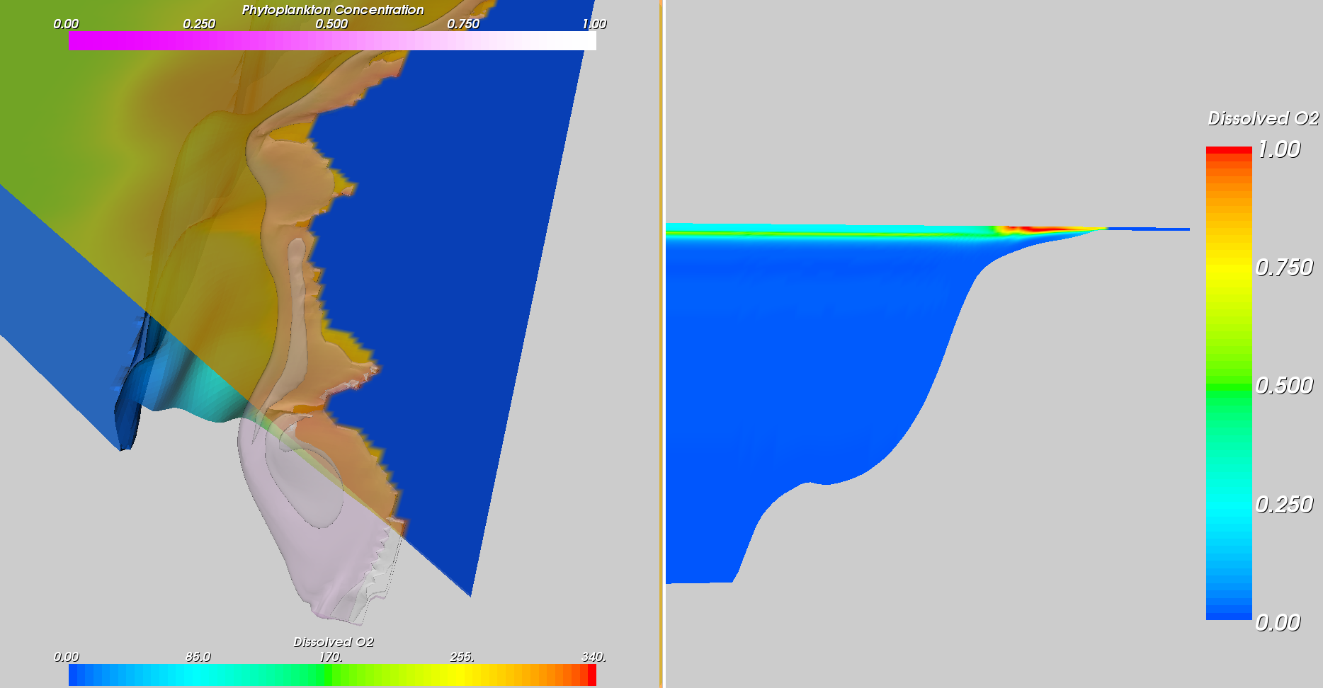
- 1.png
- This visualization uses a combination of iso-surfaces of phytoplankton concentration and O2 saturation of the domain.
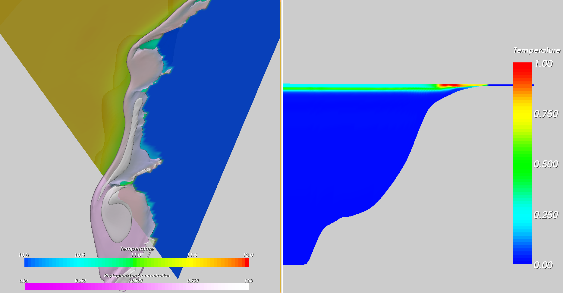
- 2.png
- Same as above only using Temperature instead of O2 saturation
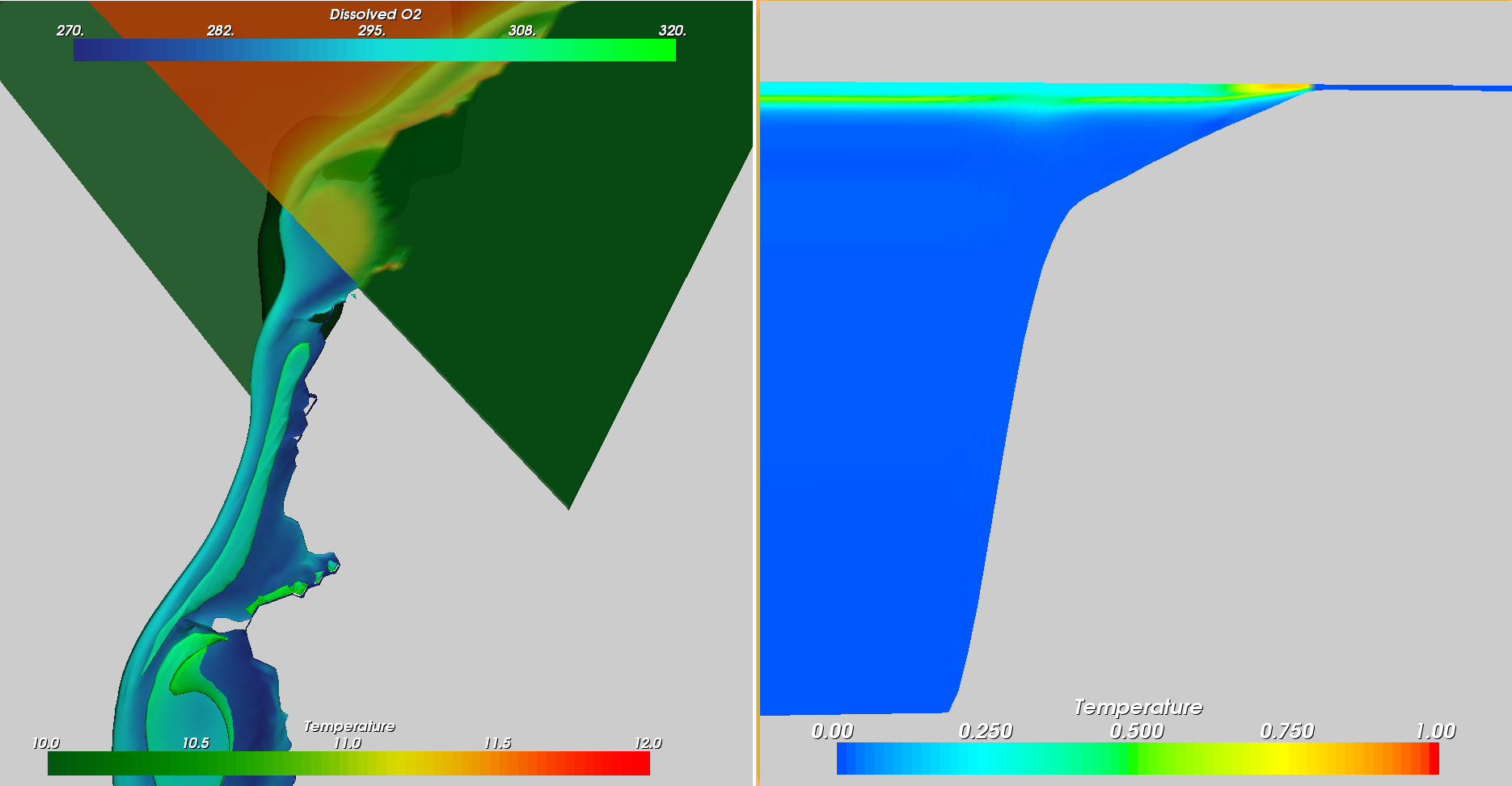
- 3.png
- Using the same iso-surfaces extracted in the above visualizations, we have loaded the O2 saturation scalar field and determined the values of this field on the phytoplankton concentration surfaces. Additionally, the entire domain is shown using an interactive cutting plane that determines the value of the 2D slice visualization as before.
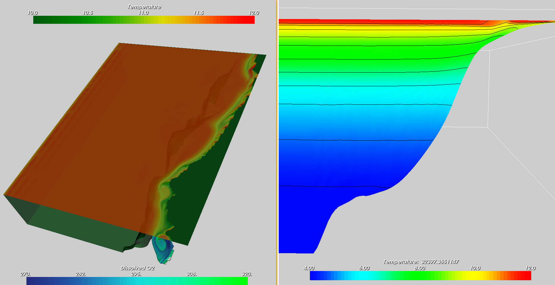
- 4.png
- Improving on the previous visualization, I am now providing equally spaced contours of the domain in the 2D slice-based visualization. This provides a much more intuitive visualization of the scalar field. Additionally, while the large 3D domain uses a relatively narrow range of the present scalar values for the colormap, I have increased this range for the 2D case. This provides a more complete visualization of the depth-based components present in the slices while accentuating surface variations in the 3D domain. I have also included the location of each slice in the dataset coordinates in the scalar bar associated with the 2D slice.
Software
- VisTrails
- Mac Binary
- Windows Binary .zip
- .vt files
- Particle Tracer
- Windows Binary
- Particle Tracer Files
- Timestep 1
- Timestep 2
Upcoming Visualizations
Particle tracing for dynamic vector field visualizations
I'm having a small issue generating the appropriate vector field from the netCDF files I have. This is due to the fact that each component of the vector exists in a different coordinate space. From some research I've done, it seems like it's based on an Arakawa C Grid. This is not a game-stopping problem, but will take some time to get things figured out. This will be an important question to be resolved in my conversations with Yvette later today (Thurs. May 28). For now, I am planning on extracting 3 different scalar fields (each with its own coordinate system) and then interpolating these values onto the domain of the scalars (the rho-grid) to coalesce the data.
I'm not entirely sure how to generate the appropriate vector field, and at first this will be further limited by the data type - the visualization software requires regular grids instead of curvilinear ones as we have. There are several possible fixes to this:
- Generate a large regular grid by embedding the curvilinear grid in a regularly gridded space. This is computationally expensive, but need only be done once per time-step and can be done with relatively little development effort - this will be the first step.
- Generate a transformation function to apply to the regular grid as a post-processing step. This is better than the first one, although more time-consuming.
- Modify the renderer to respect curvilinear grids. This is the preferred option, but takes the most time.