Parameter Exploration
While exploring workflows, one critical task is tweaking parameter values to improve simulations or visualizations. VisTrails contains an integrated parameter exploration interface that lets you thoroughly explore the parameter space and quickly identify the desired settings. By binding parameters to a range of values, you can generate a collection of results without having to tediously edit the workflow.
VisTrails Parameter Exploration is Spreadsheet-aware, so you can map the intermediate results from explorations into cells of the Spreadsheet. Because the Spreadsheet provides a multi-view interface that makes efficient use of screen space, you can quickly compare the results of different parameter settings. The changes in parameters can be displayed across rows, columns, and sheets. In addition, parameters can be explored across timesteps, and then displayed in the Spreadsheet as animations. This could be used, for example, to show how pathological tissues and tumors are affected by radiation treatment in a series of scans.
Creating a Parameter Exploration
To access VisTrails Parameter Exploration for the currently-active workflow, click on the Exploration button in the VisTrails toolbar.
The Parameter Exploration view starts out with a blank central canvas wherein exploration parameters can be set up. On the right side of the window, there are a variety of panels that control aspects of the exploration.
The Set Methods panel contains the list of parameters that can be explored, the Annotated Pipeline panel displays the workflow to be explored and helps resolve ambiguities for parameter settings, and the Spreadsheet Virtual Cell aids users in laying out exploration results in the spreadsheet.
To add parameters to an exploration, simply drag the corresponding method from the Set Methods panel to the center canvas. To reduce clutter, this panel only shows the methods for which parameters were assigned values in the Pipeline view. See Chapter Creating and Modifying Workflows for instructions on adding methods and parameters to a module.
After dragging a method to the exploration canvas, you can, for each parameter, set the collection of values to be explored and the direction in which to explore (Figure Setting values for parameter exploration). By default, intermediate parameter values are set via linear interpolation. We will discuss other options later.
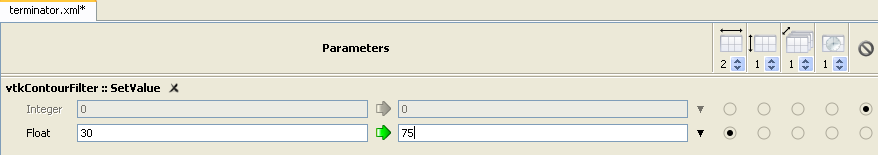
Setting values for parameter exploration.
The five column headings in the upper-right corner of the main canvas control how the results of the parameter exploration will be displayed in the Spreadsheet. From left to right, the five controls determine:
 |
exploration in the ‘x’ direction |
 |
exploration in the ‘y’ direction |
 |
exploration in the ‘z’ direction |
 |
exploration in time |
 |
none; do not vary this parameter |
The spinner beneath each of these icons lets you control the number of parameter values to be explored in that direction. For each parameter, you must select one of the radio buttons corresponding to a direction of exploration (‘x’, ‘y’, ‘z’, time, or none). Note that choosing the final column disables exploration for that parameter.
To run a parameter exploration, click the Execute button in the VisTrails toolbar or select Execute from the Workflow menu.
We now reinforce the above discussion with three examples, motivated by the problem of finding isosurfaces for medical imaging. In the examples that follow, we’ll look at determining the interfaces between different types of tissue captured by CT scans.
Try it now!
To begin, load the terminator.vt vistrail, select the “Isosurface” node in the version tree, and switch to parameter exploration. From the Pipeline Methods panel, click and drag the SetValue method of the vtkContourFilter module to the center canvas.
We’d like to compare different values for the isosurfaces so change the start and end values of the “Float” parameter to “30” and “75”. Since side-by-side visualization will look better on most monitors, select the radio button below the ‘x’ dimension control, and increase the value of the control to 2 (see Figure Setting values for parameter exploration). Execute the exploration and switch to the Spreadsheet to view the results. They should match Figure Parameter Exploration of two isovalues.... (Open result)
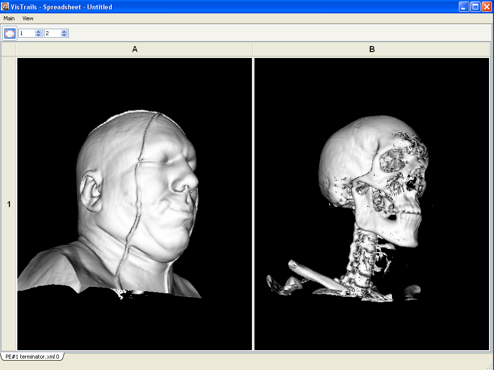
Parameter Exploration of two isovalues as displayed in the Spreadsheet.
Next Step!
While these two isovalues show interesting features, we may wish to examine other intermediate isosurfaces. To do so, switch back to the main VisTrails window and increase the number of results to generate in the ‘x’ direction to four. VisTrails will calculate the intermediate values via linear interpolation, and your execution of this new exploration should match Figure Parameter Exploration of four isovalues.... (Open result)
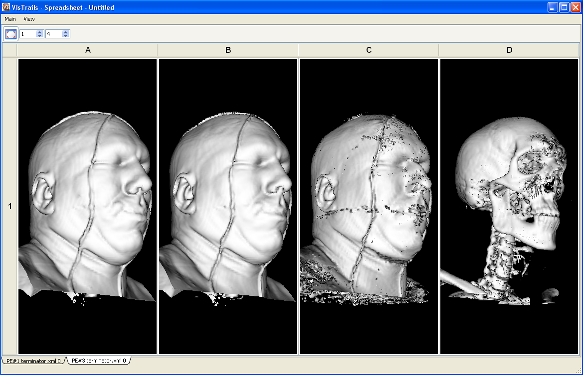
Parameter Exploration of four isovalues as displayed in the Spreadsheet.
In our next example, we demonstrate how multiple parameter values can be explored simultaneously. We will use both X and Y exploration directions to change the values of two parameters at the same time in the same spreadsheet.
Try it now!
In the terminator.vt example vistrail, make sure you’re working with the “Isosurface” version of the workflow, then go to the Pipeline view. Add the module vtkImageResample to the pipeline, and insert it between vtkStructuredPointsReader and vtkContourFilter, connecting the output of the reader to input of the resampler and the output of the resampler to the input of the contour filter as shown in Figure Inserting a vtkImageResample module.... Finally, select the vtkImageResample module and set the SetAxisMagnificationFactor to 0 and 0.2. See Chapter Creating and Modifying Workflows for reminders on how to accomplish these tasks. After modifying the workflow, switch back to the Exploration view. Inside the Set Methods panel, select the SetValue method from the vtkContourFilter module, and drag it to the center canvas. Also select the SetAxisMagnificationFactor method from the vtkImageResample module and drag it to the canvas. Set the values as in the previous example, and set the range of the “Float” parameter of “SetAxisMagnificationFactor” to start at 0.2 and end at 1.0. Also, set the magnification factor to vary over the ‘y’ direction. Finally, set the exploration to generate 16 results, four in the ‘x’ direction, and four in the ‘y’ direction. Your exploration setup should match Figure Setting up parameter exploration, and after executing, you should see a result that resembles Figure Resulting spreadsheet. Notice that the isosurface changes from left to right while the images have less artifacts as the magnification factor approaches 1.0 from top to bottom. (Open result)
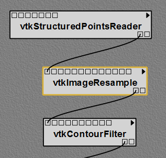
Inserting a vtkImageResample module into the “terminator.vt” example pipeline.
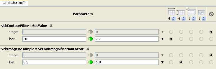
Setting up parameter exploration.
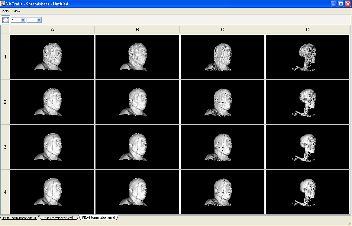
Resulting spreadsheet.
Our third example shows how to create an animation by exploring parameter values in time, rather than in ‘X’ or ‘Y’.
Try it now!
To create an animation, we’ll use the same terminator example (make sure that you have the “Isosurface” version selected). Follow the same steps as in the first example, but this time, use the range from 30 to 80 and select “time” as the dimension to explore, setting the number of results to generate to 7. See Figure Setting up parameter exploration to check your settings. After executing, the Spreadsheet will show a single cell, but if you select that cell, you will be able to click the Play button in the toolbar. You should see an animation where each frame is the result of choosing a different isovalue. A sample frame is displayed in Figure One frame from the resulting animation. (Open result)
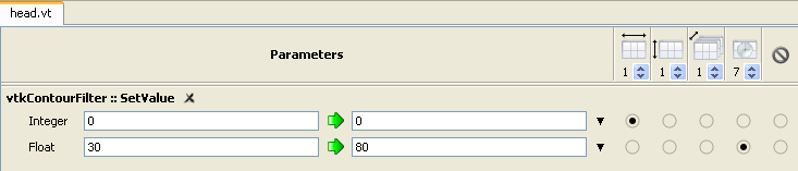
Setting up parameter exploration.
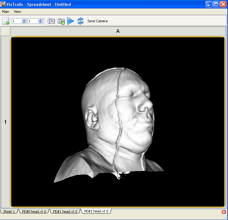
One frame from the resulting animation.
Alternatives to Linear Interpolation
In each of the examples above, we used linear interpolation to vary the parameter values in ‘X’ and ‘Y’ and time. However, linear interpolation is only one of three methods for exploring a range of parameter values. The other two are to iterate through a simple list of values, or use a user-defined function. You can choose the desired method from the drop-down menu on the right side of the parameter input field (Figure Choose from linear interpolation, list, or user-defined function). For linear interpolation, the starting and ending values must be specified; for a list, the entire comma-separated list must be specified, and for a user-defined function, a Python function must be specified. For the list and user-defined functions, you can access an editor via the ‘...’ button. (See Figure Editors for lists of values for examples of the list editor and Python editor widgets.) As an alternative to the list editor, you can manually enter a list using Python notation; for example, [30, 36, 45, 75]. As before, to set the direction in which to explore a given parameter, simply select the radio button in the column for the specified direction.

Choose from linear interpolation, list, or user-defined function.
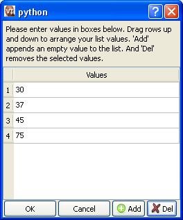
Editors for lists of values.
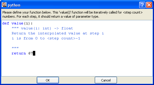
Editors for user-defined functions.
In both the Set Methods and Annotated Pipeline panels, you may see numbered red circles. See Figure The panels of the Parameter Exploration window... for an example of what this looks like. These circles appear when there is more than one module of a given type in a workflow. For each type satisfying this criteria, the instances are numbered and displayed so that you can identify which part of the pipeline a module in the Set Methods panel corresponds to.
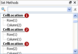
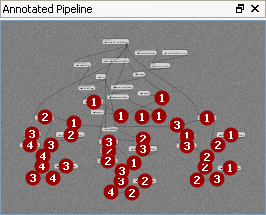
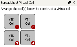
The panels of the Parameter Exploration window. Set Methods (Top) will appear in the right panel and the others will be on the left. The numbered red circles in the Annotated Pipeline (Middle) distinguish duplicate modules, and the cells in the Spreadsheet Virtual Cell (Bottom) determine the layout for spreadsheet results.
Saving Parameter Explorations
New parameter explorations are saved automatically when they are executed. The inspector (below) has buttons for moving back and forward through the history of parameter explorations. Explorations can be tagged with a name, which will make them visible in the workspace view.
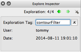
The parameter exploration inspector
“Virtual Cell” Layout
As stated earlier, the Spreadsheet provides integrated support
for parameter explorations. Each of the directions of exploration
corresponds to a visual dimension in the spreadsheet: the ‘x’
direction corresponds to columns; the ‘y’ direction to rows; the
‘z’ direction to sheets; and time to animations. However, when
a workflow already outputs to more than one cell, you can layout the
group of cells as it will be replicated during the exploration. For
example, given a workflow with two output cells and an exploration for
three parameter values in the ‘x’ direction, the resulting
spreadsheet could be  or
or  . The
Spreadsheet Virtual Cell panel controls the layout of
the pattern. Drag and drop cells to position them. See
Figures The panels of the Parameter Exploration window (Bottom) and Results of the Virtual Cell arrangement
for an example.
. The
Spreadsheet Virtual Cell panel controls the layout of
the pattern. Drag and drop cells to position them. See
Figures The panels of the Parameter Exploration window (Bottom) and Results of the Virtual Cell arrangement
for an example.
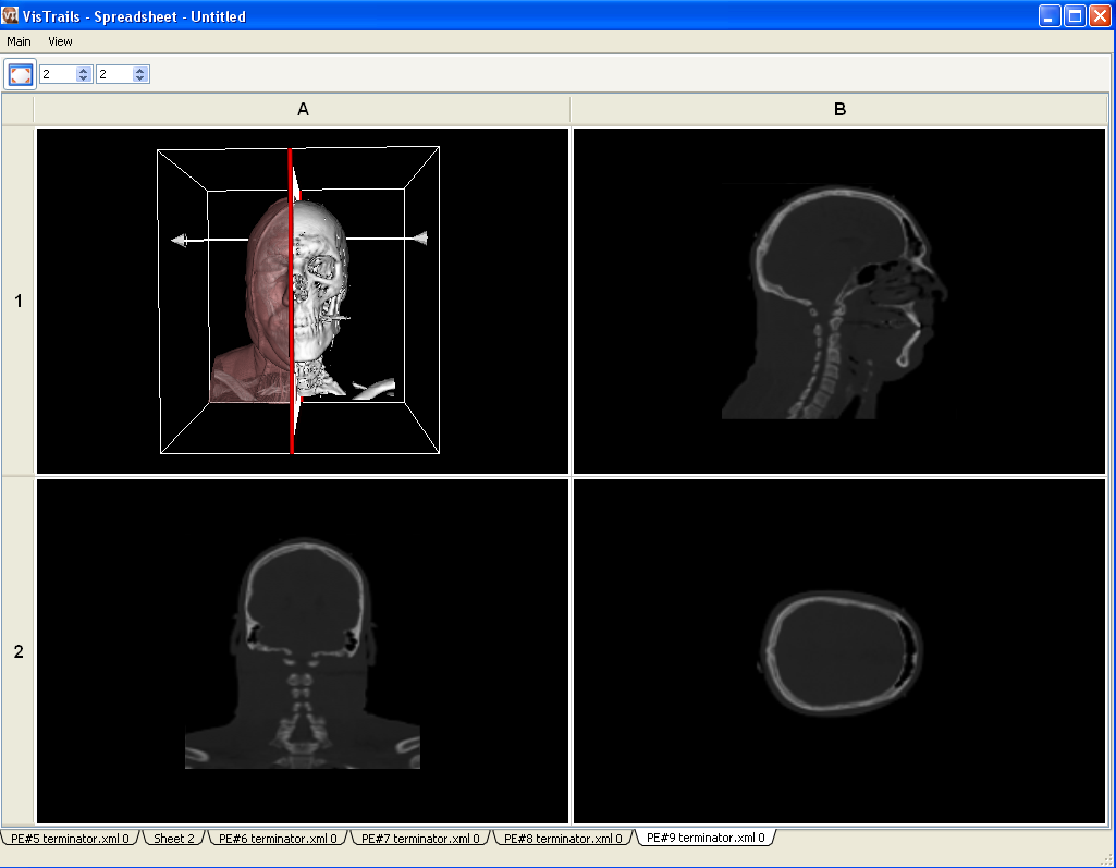
Results of the Virtual Cell arrangement.