User:Tohline/ThreeDimensionalConfigurations/ChallengesPt2
Challenges Constructing Ellipsoidal-Like Configurations (Pt. 2)
This chapter extends an accompanying chapter titled, Construction Challenges (Pt. 1). The focus here is on an SCF technique that will incorporate specification of a Lagrangian flow-flied.

|
|---|
| | Tiled Menu | Tables of Content | Banner Video | Tohline Home Page | |
Motivation
In a separate discussion, we have shown that, as viewed from a frame that "tumbles" with the (purple) body of a Type 1 Riemann ellipsoid, each Lagrangian fluid element moves along an elliptical path in a plane that is tipped by an angle <math>~\theta</math> (about the x-axis of the body). As viewed from the (primed) coordinates associated with this tipped plane, by definition, z' = 0, and the planar orbit is defined by the expression,
|
<math>~1</math> |
<math>~=</math> |
<math>~\biggl(\frac{x'}{x_\mathrm{max}} \biggr)^2 + \biggl(\frac{y' - y_0}{y_\mathrm{max}} \biggr)^2 \, .</math> |
As a function of time, the x'-y' coordinates and associated velocity components of each particle are given by the expressions,
|
<math>~x'</math> |
<math>~=</math> |
<math>~x_\mathrm{max}\cos(\varphi t)</math> |
and, |
<math>~y' - y_0</math> |
<math>~=</math> |
<math>~y_\mathrm{max}\sin(\varphi t) \, ,</math> |
|
<math>~\dot{x}'</math> |
<math>~=</math> |
<math>~- x_\mathrm{max}~ \varphi \cdot \sin(\varphi t)</math> |
and, |
<math>~\dot{y}' </math> |
<math>~=</math> |
<math>~y_\mathrm{max}~\varphi \cdot \cos(\varphi t) \, .</math> |
Here we provide analytic expressions for these various quantities — <math>~x_\mathrm{max}, y_\mathrm{max}, y_0, \varphi</math> — in terms of the properties of any chosen Type 1 Riemann ellipsoid.
Intersection of Tipped Plane With Ellipsoid Surface
In a an early subsection of the accompanying discussion, we have
Example Equilibrium Model
These key parameters have been drawn from [EFE] Chapter 7, Table XIII (p. 170):
| <math>~a = a_1 = 1</math> |
| <math>~b = a_2 = 1.25</math> |
| <math>~c = a_3 = 0.4703</math> |
| <math>~\Omega_2 = 0.3639</math> |
| <math>~\Omega_3 = 0.6633</math> |
| <math>~\zeta_2 = - 2.2794</math> |
| <math>~\zeta_3 = - 1.9637</math> |
As a consequence — see an accompanying discussion for details — the values of other parameters are …
| Example Values | ||||||
|
<math>~\tan\theta </math> |
<math>~=</math> |
<math>~- \frac{\zeta_2 }{ \zeta_3 } \biggl[ \frac{a^2 + b^2}{a^2 + c^2} \biggr]\frac{c^2}{b^2} = -0.344793</math> |
<math>~~ \theta =</math> |
<math>~- 19.0238^\circ</math> |
||
|
<math>~ \Lambda </math> |
<math>~\equiv</math> |
<math> \biggl[ \frac{a^2}{a^2 + b^2} \biggr] \zeta_3 \cos\theta - \biggl[ \frac{a^2}{a^2 + c^2} \biggr] \zeta_2 \sin\theta </math> |
<math>~\Lambda =</math> |
<math>~-1.332892 </math> |
||
|
<math>~ \frac{y_0}{z_0} </math> |
<math>~=</math> |
<math> \biggl[ \frac{a^2}{a^2 + c^2} \biggr] \frac{\zeta_2}{\Lambda} </math> |
<math>~\frac{y_0}{z_0} =</math> |
<math>~+ 1.400377</math> |
||
|
<math>~ \frac{x_\mathrm{max}}{ y_\mathrm{max} } </math> |
<math>~=</math> |
<math>~ \biggl\{ \Lambda \biggl[ \frac{a^2 + b^2}{b^2} \biggr] \frac{\cos\theta}{\zeta_3} \biggr\}^{1 / 2} </math> |
<math>~\frac{x_\mathrm{max}}{y_\mathrm{max}} =</math> |
<math>~+ 1.025854</math> |
||
|
<math>~ \varphi </math> |
<math>~=</math> |
<math>~ \biggl\{ \Lambda \biggl[ \frac{b^2}{a^2 + b^2} \biggr] \frac{\zeta_3 }{\cos\theta} \biggr\}^{1 / 2} </math> |
<math>~\varphi =</math> |
<math>~+1.299300</math> |
||
COLLADA-Based Representation
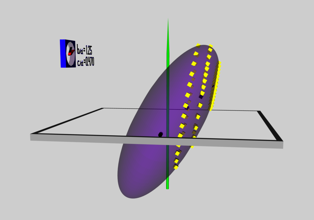
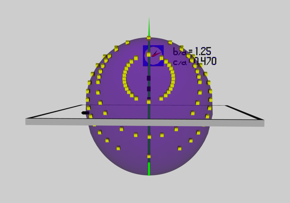
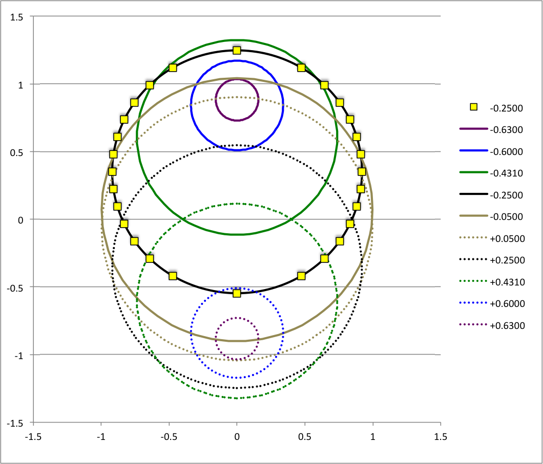
As has been described in an accompanying discussion of Riemann Type 1 ellipsoids, we have used COLLADA to construct an animated and interactive 3D scene that displays in purple the surface of an example Type I ellipsoid; panels a and b of Figure 1 show what this ellipsoid looks like when viewed from two different perspectives. (As a reminder — see the explanation accompanying Figure 2 of that accompanying discussion — the ellipsoid is tilted about the x-coordinate axis at an angle of 61.25° to the equilibrium spin axis, which is shown in green.) Yellow markers also have been placed in this 3D scene at each of the coordinate locations specified in the table that accompanies that discussion. From the perspective presented in Figure 3b, we can immediately identify three separate, nearly circular trajectories; the largest one corresponds to our choice of z0 = -0.25, the smallest corresponds to our choice of z0 = -0.60, and the one of intermediate size correspond to our choice of z0 = -0.4310. When viewed from the perspective presented in Figure 1a, we see that these three trajectories define three separate planes; each plane is tipped at an angle of θ = -19.02° to the untilted equatorial, x-y plane of the purple ellipsoid.
See Also

|
|---|
|
© 2014 - 2021 by Joel E. Tohline |


