User:Tohline/SSC/Stability/Isothermal
Radial Oscillations of Pressure-Truncated Isothermal Spheres

|
|---|
| | Tiled Menu | Tables of Content | Banner Video | Tohline Home Page | |
Overview
Both Ebert (1955) and Bonnor (1956) showed that, when presented in a pressure-volume diagram, the equilibrium sequence of pressure-truncated isothermal spheres displays an astrophysical interesting turning point. This turning point signifies that there is a critical external pressure above which no equilibrium configurations exist. As we have summarized in a related discussion, Bonnor furthermore showed that this turning point lies along the equilibrium sequence approximately halfway between configurations that have a truncation radius of <math>~\xi_e = 6</math> and <math>~\xi_e = 7</math>, and that it is identified by the model whose isothermal Lane-Emden function, <math>~\psi(\xi)</math>, exhibits the property,
|
<math>~\biggl[e^{\psi} \biggl( \frac{d\psi}{d\xi}\biggr)^2\biggr]_\mathrm{surf}</math> |
<math>~=</math> |
<math>~2 \, ,</math> |
at its surface. At the time, it was left unanswered whether this turning point is only significant in the context of secular evolution along the equilibrium sequence, or whether it is associated with the onset of a dynamical instability. As far as we have been able to determine, Yabushita (1968) was the first to point out that, in principle, the relative [dynamical] stability of this "turning point" model can be ascertained by using linear stability analysis techniques to examine the sign of <math>~\lambda_0^2</math>, which is the square of the eigenfrequency of the configuration's fundamental radial mode of oscillation.
Yabushita's (1968) stability analysis showed that the marginally [dynamically] unstable model does lie between <math>~\xi_e = 6</math> and <math>~\xi_e = 7</math>. This was confirmed by the follow-up stability analysis published by Taff & Van Horn (1974). As is demonstrated in subsequent subsections of this chapter, we have reproduced in detail the subset of Taff & Van Horn's results that are directly related to this stability question. Extending the application of these standard linear stability analysis techniques, we have furthermore determined that the marginally unstable model has a truncation radius of,
<math>~\xi_e \approx 6.4510534 \, ,</math>
and that, for this specific model,
|
<math>~\biggl[e^{\psi} \biggl( \frac{d\psi}{d\xi}\biggr)^2\biggr]_\mathrm{surf}</math> |
<math>~\approx</math> |
<math>~1.9999588 \, .</math> |
Hence, to a high degree of precision, it appears as though the equilibrium configuration that sits at the limiting-pressure turning point can also be identified as the model along the equilibrium sequence that separates dynamically stable configurations from dynamically unstable ones.
Groundwork
Equilibrium Model
Review
In an accompanying discussion, while reviewing the original derivations of Ebert (1955) and Bonnor (1956), we have detailed the equilibrium properties of pressure-truncated isothermal spheres. These properties have been expressed in terms of the isothermal Lane-Emden function, <math>~\psi(\xi)</math>, which provides a solution to the governing,
Isothermal Lane-Emden Equation
|
A parallel presentation of these details can be found in §2 — specifically, equations (2.4) through (2.10) — of Yabushita (1968). Each of Yabushita's key mathematical expressions can be mapped to ours via the variable substitutions presented here in Table 1.
|
Table 1: Mapping from Yabushita's (1968) Notation to Ours |
||||||
| Yabushita's (1968) Notation: | <math>~x</math> | <math>~\psi</math> | <math>~\mu</math> | <math>~M</math> | <math>~x_0</math> | <math>~p_0</math> |
| Our Notation: | <math>~\xi</math> | <math>~-\psi</math> | <math>~\bar\mu</math> | <math>~M_{\xi_e}</math> | <math>~\xi_e</math> | <math>~P_e</math> |
For example, given the system's sound speed, <math>~c_s</math>, and total mass, <math>~M_{\xi_e}</math>, the expression from our presentation that shows how the bounding external pressure, <math>~P_e</math>, depends on the dimensionless Lane-Emden function, <math>~\psi</math>, is,
|
<math>~P_e</math> |
<math>~=</math> |
<math>~\biggl( \frac{c_s^8}{4\pi G^3 M_{\xi_e}^2} \biggr) ~\xi_e^4 \biggl(\frac{d\psi}{d\xi}\biggr)^2_e e^{-\psi_e}</math> |
|
<math>~\Rightarrow ~~~ \xi_e^2 \biggl(\frac{d\psi}{d\xi}\biggr)_e e^{-(1/2)\psi_e}</math> |
<math>~=</math> |
<math>~\frac{1}{c_s^4}\biggl[ G^3 M_{\xi_e}^2 ~(4\pi P_e)\biggr]^{1 / 2} \, ,</math> |
which — see the boxed-in excerpt that follows — exactly matches Yabushita's (1968) equation (2.9), after recalling that the system's sound speed is related to its temperature via the relation,
<math>c_s^2 = \frac{\Re T}{\bar{\mu}} \, .</math>
And, our expression for the truncated configuration's equilibrium radius is,
|
<math>~R</math> |
<math>~=</math> |
<math>~\frac{GM_{\xi_e}}{c_s^2} \biggl[ \xi \biggl(\frac{d\psi}{d\xi}\biggr) \biggr]_e^{-1}</math> |
which — see the boxed-in excerpt that follows — matches Yabushita's (1968) equation (2.10).
|
Equations extracted† from p. 110 of S. Yabushita (1968)
"Jeans's Type Gravitational Instability of Finite Isothermal Gas Spheres"
MNRAS, vol. 140, pp. 109-120 © Royal Astronomical Society |
 |
|
†Layout of equations has been modified from the original publication. |
P-V Diagram
As we have discussed in a separate chapter that focuses on the structural properties of pressure-truncated Isothermal spheres, Bonnor (1956) examined the sequence of equilibrium models that is generated by varying the truncation radius over the range, <math>~0 < \xi_e < \infty</math>. In a diagram that shows how <math>~P_e(\xi_e)</math> varies with equilibrium volume, <math>~V(\xi_e) \propto R^3</math>, Bonnor noticed that there is a pressure above which no equilibrium configurations exist. The original P-V diagram published by Bonnor (1956) has been reproduced here, in the left-hand panel of our Figure 1. The right-hand panel of Figure 1 shows the same equilibrium sequence, as generated from our numerical integration of the isothermal Lane-Emden equation; we have adopted Whitworth's normalizations, <math>~P_\mathrm{rf}</math> and <math>~V_\mathrm{rf}</math>.
Figure 1: Bonnor's P-V Diagram (see accompanying discussion for details)
|
Figure extracted from p. 355 of W. B. Bonnor (1956)
"Boyle's Law and Gravitational Instability"
MNRAS, vol. 116, pp. 351 - 359 © Royal Astronomical Society |
Bonnor's (1956) equilibrium sequence, but as generated from our numerical integration of the isothermal Lane-Emden equation; in our plot, we have adopted Whitworth's (1981) normalizations, <math>~P_\mathrm{rf}</math> and <math>~V_\mathrm{rf}</math>. |
 |
 |
As is discussed below, in separate studies, Yabushita (1968) and Taff & Van Horn (1974) examined the lowest-order modes of radial oscillations that arise in pressure-truncated isothermal spheres. In both studies, numerical techniques were used to solve the eigenvalue problem associated with the isothermal LAWE, as derived below. The nine individual equilibrium models that were studied by Taff & Van Horn are identified by the nine small, filled circular markers along the sequence that has been displayed in the right-hand panel of our Figure 1; as labeled, they correspond to models with <math>~\xi_e</math> = 2, 3, 4, 5, 6, 7, 8, 9, and 10. Earlier, Yabushita studied the oscillation modes of three of these same configurations; specifically, the models with <math>~\xi_e</math> = 6, 7, and 8, which straddle the location along the equilibrium sequence of the model associated with the pressure maximum (the turning point labeled "A" in Bonnor's P-V diagram).
Other Properties
Also, as has been summarized in our accompanying discussion of the equilibrium properties of pressure-truncated isothermal spheres, we have,
|
<math>~r_0 </math> |
<math>~=</math> |
<math>~\biggl( \frac{c_s^2}{4\pi G \rho_c} \biggr)^{1/2} \xi \, ;</math> |
|
<math>~P_0 = c_s^2 \rho_0 </math> |
<math>~=</math> |
<math>~(c_s^2 \rho_c) e^{-\psi} \, ;</math> |
|
<math>~M_r </math> |
<math>~=</math> |
<math>~\biggl( \frac{c_s^6}{4\pi G^3 \rho_c} \biggr)^{1/2} \biggl[ \xi^2 \frac{d\psi}{d\xi} \biggr] \, .</math> |
Hence, for isothermal configurations,
|
<math>~g_0 \equiv \frac{GM_r}{r_0^2}</math> |
<math>~=</math> |
<math>~G\biggl( \frac{c_s^6}{4\pi G^3 \rho_c} \biggr)^{1/2} \biggl[ \xi^2 \frac{d\psi}{d\xi} \biggr] \biggl[ \biggl( \frac{c_s^2}{4\pi G \rho_c} \biggr)^{1/2} \xi\biggr]^{-2}</math> |
|
|
<math>~=</math> |
<math>~c_s^2 \biggl( \frac{4\pi G \rho_c}{c_s^2} \biggr)^{1 / 2} \biggl( \frac{d\psi}{d\xi} \biggr) \, . </math> |
Linearized Wave Equation
In our introductory discussion of techniques that facilitate linear stability analyses, we derived what we now repeatedly refer to as the "key" form of the
LAWE: Linear Adiabatic Wave (or Radial Pulsation) Equation
|
|
<math>~ \frac{d^2x}{dr_0^2} + \biggl[\frac{4}{r_0} - \biggl(\frac{g_0 \rho_0}{P_0}\biggr) \biggr] \frac{dx}{dr_0} + \biggl(\frac{\rho_0}{\gamma_\mathrm{g} P_0} \biggr)\biggl[\omega^2 + (4 - 3\gamma_\mathrm{g})\frac{g_0}{r_0} \biggr] x = 0 </math> |
[P00], Vol. II, §3.7.1, p. 174, Eq. (3.144)
Here we review two published articles that have presented a partial analysis of radial modes of oscillation in pressure-truncated isothermal spheres. The analyses presented in both of these papers, effectively, employ this key wave equation, but the authors of these articles present it in different forms.
Yabushita (1968)
The linearized wave equation that Yabushita (1968) used to examine the radial pulsation modes of pressure-truncated isothermal spheres is displayed in the following, boxed-in image:
|
Equation extracted from p. 111 of S. Yabushita (1968)
"Jeans's Type Gravitational Instability of Finite Isothermal Gas Spheres"
MNRAS, vol. 140, pp. 109-120 © Royal Astronomical Society |
 |
This equation can be obtained straightforwardly through a strategic combination of three of the following four linearized principal governing equations that we have derived in our accompanying, broad introductory discussion of linear stability analyses, namely,
|
Linearized Linearized Linearized <math> P_1 = \biggl( \frac{dP}{d\rho} \biggr)_0 \rho_1\, , </math> Linearized <math> \nabla^2 \Phi_1 = 4\pi G \rho_1\, . </math> |
Taking the partial time-derivative of the linearized equation of continuity gives,
|
<math>~- \nabla\cdot \frac{\partial \vec{v}}{\partial t} </math> |
<math>~=</math> |
<math>~\frac{1}{\rho_0}\frac{\partial^2 \rho_1}{\partial t^2} + \frac{\nabla\rho_0}{\rho_0} \cdot \frac{\partial\vec{v}}{\partial t} \, ;</math> |
and, taking the divergence of the linearized Euler equation gives,
|
<math>~-\nabla\cdot \frac{\partial \vec{v}}{\partial t} </math> |
<math>~=</math> |
<math>~\nabla^2 \Phi_1 + \nabla\cdot \biggl[\frac{1}{\rho_0} \nabla P_1\biggr] - \nabla \cdot \biggl[ \frac{\rho_1}{\rho_0^2} \nabla P_0 \biggr] \, .</math> |
Combining the two, then making two substitutions using (1) the linearized Poisson equation and (2) the linearized Euler equation, we have,
|
<math>~\frac{\partial^2 \rho_1}{\partial t^2} + \nabla\rho_0 \cdot \frac{\partial\vec{v}}{\partial t} </math> |
<math>~=</math> |
<math>~\rho_0 \nabla^2 \Phi_1 + \rho_0 \nabla\cdot \biggl[\frac{1}{\rho_0} \nabla P_1\biggr] - \rho_0\nabla \cdot \biggl[ \frac{\rho_1}{\rho_0^2} \nabla P_0 \biggr] </math> |
|
<math>~\Rightarrow ~~~ \frac{\partial^2 \rho_1}{\partial t^2} + \nabla\rho_0 \cdot \biggl[ - \nabla\Phi_1 - \frac{1}{\rho_0} \nabla P_1 + \frac{\rho_1}{\rho_0^2} \nabla P_0 \biggr] </math> |
<math>~=</math> |
<math>~4\pi G \rho_0 \rho_1 + \nabla^2 P_1 + \rho_0 \nabla P_1 \cdot \nabla \biggl(\frac{1}{\rho_0} \biggr) - \rho_0\nabla \cdot \biggl[ \frac{\rho_1}{\rho_0^2} \nabla P_0 \biggr] \, .</math> |
Rearranging terms, and using the replacement equilibrium relation, <math>~\nabla P_0 = - \rho_0\nabla\Phi_0</math>, gives,
|
<math>~ \frac{\partial^2 \rho_1}{\partial t^2} - \nabla^2 P_1 - 4\pi G \rho_0 \rho_1 - \nabla\rho_0\cdot\nabla\Phi_1 </math> |
<math>~=</math> |
<math>~ \frac{\nabla\rho_0}{\rho_0} \cdot \biggl[ \nabla P_1 + \rho_1 \nabla \Phi_0 \biggr] + \rho_0 \nabla P_1 \cdot \nabla \biggl(\frac{1}{\rho_0} \biggr) + \rho_0\nabla \cdot \biggl[ \frac{\rho_1}{\rho_0} \nabla \Phi_0 \biggr] </math> |
|
|
<math>~=</math> |
<math>~ \frac{\nabla\rho_0}{\rho_0} \cdot \biggl[ \nabla P_1 \biggr] + \frac{\rho_1}{\rho_0} \biggl[ \nabla\rho_0\cdot \nabla \Phi_0 \biggr] - \frac{1}{\rho_0} \nabla P_1 \cdot \nabla \rho_0 + \rho_0 \nabla \Phi_0 \cdot \nabla \biggl[ \frac{\rho_1}{\rho_0} \biggr] + \rho_1\nabla^2 \Phi_0 </math> |
|
|
<math>~=</math> |
<math>~ \frac{\rho_1}{\rho_0} \biggl[ \nabla\rho_0\cdot \nabla \Phi_0 \biggr] - \frac{\rho_1}{\rho_0} \biggl[ \nabla \Phi_0 \cdot \nabla\rho_0\biggr] + \nabla \Phi_0 \cdot \nabla \rho_1 + 4\pi G \rho_0 \rho_1 </math> |
|
<math>~\Rightarrow ~~~ \frac{\partial^2 \rho_1}{\partial t^2} - \nabla^2 P_1 - 8\pi G \rho_0 \rho_1 - \nabla\rho_0\cdot\nabla\Phi_1 - \nabla \Phi_0 \cdot \nabla \rho_1 </math> |
<math>~=</math> |
<math>~0 \, .</math> |
This is identical to Yabushita's (1968) equation (2.12). Letting <math>~t \rightarrow (4\pi G \rho_c)^{-1 / 2} \tau</math> and noting that <math>\rho_c = P_c/c_s^2</math>, we also have,
|
<math>~0 </math> |
<math>~=</math> |
<math>~ 4\pi G \rho_c^2 ~\biggl\{ \frac{\partial^2}{\partial \tau^2}\biggl(\frac{\rho_1}{\rho_c}\biggr) - \frac{1}{4\pi G \rho_c^2}\nabla^2 P_1 - 2 \biggl(\frac{\rho_0}{\rho_c}\biggr) \biggl(\frac{\rho_1}{\rho_c}\biggr) - \frac{1}{4\pi G \rho_c^2} \nabla\rho_0\cdot\nabla\Phi_1 - \frac{1}{4\pi G \rho_c^2} \nabla \Phi_0 \cdot \nabla \rho_1 \biggr\} </math> |
|
<math>~\Rightarrow ~~~ 0</math> |
<math>~=</math> |
<math>~ \frac{\partial^2}{\partial \tau^2}\biggl(\frac{\rho_1}{\rho_c}\biggr) - \frac{c_s^2}{4\pi G \rho_c}\nabla^2 \biggl(\frac{P_1}{P_c}\biggr) - 2\biggl(\frac{\rho_0}{\rho_c}\biggr) \biggl(\frac{\rho_1}{\rho_c}\biggr) - \frac{c_s^2}{4\pi G \rho_c} \nabla\biggl( \frac{\rho_0}{\rho_c}\biggr) \cdot \nabla \biggl( \frac{\Phi_1 }{c_s^2}\biggr) - \frac{c_s^2}{4\pi G \rho_c} \nabla \biggl( \frac{\Phi_0}{c_s^2}\biggr) \cdot \nabla \biggl(\frac{ \rho_1}{\rho_c} \biggr) </math> |
|
|
<math>~=</math> |
<math>~ \frac{\partial^2}{\partial \tau^2}\biggl(\frac{\rho_1}{\rho_c}\biggr) - \nabla_\xi^2 \biggl(\frac{P_1}{P_c}\biggr) - 2\biggl(\frac{\rho_0}{\rho_c}\biggr) \biggl(\frac{\rho_1}{\rho_c}\biggr) - \nabla_\xi\biggl( \frac{\rho_0}{\rho_c}\biggr) \cdot \nabla_\xi \biggl( \frac{\Phi_1 }{c_s^2}\biggr) - \nabla_\xi \biggl( \frac{\Phi_0}{c_s^2}\biggr) \cdot \nabla_\xi \biggl(\frac{ \rho_1}{\rho_c} \biggr) \, , </math> |
where, in this last step, we have switched from the radial coordinate, <math>~r</math>, to the dimensionless coordinate, <math>~\xi \equiv r (4\pi G\rho_c/c_s^2)^{1 / 2}</math>. This matches Yabushita's (1968) equation (2.15).
Now, in principle, we can rewrite this linearized wave equation entirely in terms of the density perturbation by recognizing that, from the isothermal equation of state,
<math>~\frac{P_1}{P_c} = \frac{\rho_1}{\rho_c}</math>;
and from the Poisson equation,
|
<math>~\nabla^2\Phi_1 = 4\pi G \rho_1</math> |
<math>~\Rightarrow</math> |
<math>~\nabla_\xi^2 \biggl( \frac{\Phi_1}{c_s^2} \biggr) = \frac{\rho_1}{\rho_c} \, .</math> |
But this does not work directly because our just-derived, governing linearized wave equation contains the term, <math>~\nabla_\xi \Phi_1</math>, rather than, <math>~\nabla_\xi^2 \Phi_1</math>. Instead, following the lead of Ebert (1957), Yabushita (1968) rewrites all of the perturbed variables in terms of a new function, <math>~g(\xi)</math>, defined such that,
|
<math>~g e^{i\omega t}</math> |
<math>~\equiv</math> |
<math>~\xi^2 \frac{d}{d\xi}\biggl( \frac{\Phi_1}{c_s^2}\biggr)</math> |
in which case, from the Poisson equation, we have,
|
<math>~\frac{\rho_1}{\rho_c} </math> |
<math>~=</math> |
<math>~\frac{1}{\xi^2} \frac{d}{d\xi} \biggl[\xi^2 \frac{d}{d\xi}\biggl( \frac{\Phi_1}{c_s^2} \biggr)\biggr] </math> |
|
|
<math>~=</math> |
<math>~\frac{1}{\xi^2} \frac{dg}{d\xi} ~e^{i\omega t} \, .</math> |
This matches both equation (12) of Ebert (1957), and equation (2.17) of Yabushita (1968). The governing wave equation therefore becomes,
|
<math>~0</math> |
<math>~=</math> |
<math>~ -\omega^2 \biggl[\frac{1}{\xi^2} \frac{dg}{d\xi} \biggr] - \frac{1}{\xi^2}\frac{d}{d\xi} \biggl[ \xi^2 \frac{d}{d\xi}\biggl( \frac{1}{\xi^2} \frac{dg}{d\xi} \biggr) \biggr] - 2\biggl(\frac{\rho_0}{\rho_c}\biggr) \biggl[ \frac{1}{\xi^2} \frac{dg}{d\xi} \biggr] - \nabla_\xi\biggl( \frac{\rho_0}{\rho_c}\biggr) \cdot \frac{g}{\xi^2} - \nabla_\xi \biggl( \frac{\Phi_0}{c_s^2}\biggr) \cdot \frac{d}{d\xi} \biggl[ \frac{1}{\xi^2} \frac{dg}{d\xi}\biggr] \, . </math> |
Finally, inserting the background, equilibrium structural profiles, in particular,
|
<math>~\frac{\rho_0}{\rho_c} = e^{-\psi}</math> |
and |
<math>~\frac{\Phi_0}{c_s^2} = \psi \, ,</math> |
[NOTE: Here, and throughout this H_Book, our adopted sign convention for <math>~\psi</math> is opposite that adopted by Yabushita (1968); see is equations (2.5) and (2.6)] we have,
|
<math>~0</math> |
<math>~=</math> |
<math>~ -\omega^2 \biggl[\frac{1}{\xi^2} \frac{dg}{d\xi} \biggr] - \frac{1}{\xi^2}\frac{d}{d\xi} \biggl[ \xi^2 \frac{d}{d\xi}\biggl( \frac{1}{\xi^2} \frac{dg}{d\xi} \biggr) \biggr] + e^{-\psi } \biggl[ - \frac{2}{\xi^2} \frac{dg}{d\xi} + \frac{g}{\xi^2}\frac{d\psi}{d\xi} \biggr] - \frac{d\psi}{d\xi} \cdot \frac{d}{d\xi} \biggl[ \frac{1}{\xi^2} \frac{dg}{d\xi}\biggr] </math> |
|
|
<math>~=</math> |
<math>~ \frac{1}{\xi^2} \biggl\{ -\omega^2 \biggl[\frac{dg}{d\xi} \biggr] - \frac{d}{d\xi} \biggl[ \xi^2 \frac{d}{d\xi}\biggl( \frac{1}{\xi^2} \frac{dg}{d\xi} \biggr) \biggr] + e^{-\psi} \biggl[ -2\frac{dg}{d\xi} + g \frac{d\psi}{d\xi} \biggr] - \xi^2 \frac{d\psi}{d\xi} \cdot \frac{d}{d\xi} \biggl[ \frac{1}{\xi^2} \frac{dg}{d\xi}\biggr] \biggr\} </math> |
|
|
<math>~=</math> |
<math>~ \frac{1}{\xi^2} \biggl\{ -\omega^2 \biggl[\frac{dg}{d\xi} \biggr] + \frac{2}{\xi} \frac{d^2g}{d\xi^2} - \frac{2}{\xi^2} \frac{dg}{d\xi} - \frac{d^3g}{d\xi^3} + e^{-\psi} \biggl[ -2\frac{dg}{d\xi} + g \frac{d\psi}{d\xi} \biggr] - \frac{d\psi}{d\xi} \biggl[ - \frac{2}{\xi} \frac{dg}{d\xi} + \frac{d^2g}{d\xi^2}\biggr] \biggr\} </math> |
|
<math>~\Rightarrow ~~~ 0</math> |
<math>~=</math> |
<math>~ \omega^2 ~\frac{dg}{d\xi} + \frac{d^3g}{d\xi^3} + \frac{d^2g}{d\xi^2}\biggl[- \frac{2}{\xi} +\frac{d\psi}{d\xi} \biggl] + \frac{dg}{d\xi} \biggl[ \frac{2}{\xi^2} - \frac{2}{\xi} \cdot \frac{d\psi}{d\xi} + 2e^{-\psi} \biggr] - g \biggl[ e^{-\psi} \frac{d\psi}{d\xi} \biggr] </math> |
|
|
<math>~=</math> |
<math>~ \frac{d^3g}{d\xi^3} - B_1(\xi) \frac{d^2 g}{d\xi^2} + [B_2(\xi) + \omega^2] \frac{dg}{d\xi} + B_3(\xi) g \, ,</math> |
where,
|
<math>~B_1</math> |
<math>~=</math> |
<math>~ \biggl[\frac{2}{\xi} - \frac{d\psi}{d\xi} \biggl] </math> |
|
<math>~B_2</math> |
<math>~=</math> |
<math>~2\biggl[ \frac{1}{\xi^2} - \frac{1}{\xi} \cdot \frac{d\psi}{d\xi} + e^{-\psi} \biggr]</math> |
|
<math>~B_3</math> |
<math>~=</math> |
<math>~- \biggl[ e^{-\psi} \frac{d\psi}{d\xi} \biggr]</math> |
Taking into account that our sign convention on <math>~\psi</math> is opposite to that adopted by Ebert (1957), this last form of the governing wave equation matches his eqs. (13) and (14) when his parameter, <math>~\alpha</math>, is set to unity (isothermal condition) and the variable substitution, <math>~\lambda \leftrightarrow i\omega</math>, is made.
Now, given that,
|
<math>~\frac{d}{d\xi} \biggl[ \frac{dg}{d\xi}\biggl(- \frac{2}{\xi} +\frac{d\psi}{d\xi} \biggr) \biggl]</math> |
<math>~=</math> |
<math>~ \frac{d^2g}{d\xi^2}\biggl(- \frac{2}{\xi} +\frac{d\psi}{d\xi} \biggl) + \biggl(\frac{2}{\xi^2} +\frac{d^2\psi}{d\xi^2} \biggr) \frac{dg}{d\xi} </math> |
|
<math>~\Rightarrow ~~~ \frac{d^2g}{d\xi^2}\biggl(- \frac{2}{\xi} +\frac{d\psi}{d\xi} \biggl) </math> |
<math>~=</math> |
<math>~ \frac{d}{d\xi} \biggl[ \frac{dg}{d\xi}\biggl(- \frac{2}{\xi} +\frac{d\psi}{d\xi} \biggr) \biggl] - \frac{dg}{d\xi}\biggl(\frac{2}{\xi^2} +\frac{d^2\psi}{d\xi^2} \biggr) \, , </math> |
we can rewrite the governing wave equation as,
|
<math>~ 0</math> |
<math>~=</math> |
<math>~ \frac{d}{d\xi} \biggl\{ \omega^2 g + \frac{d^2g}{d\xi^2} + \frac{dg}{d\xi}\biggl(- \frac{2}{\xi} +\frac{d\psi}{d\xi} \biggr) \biggr\} + \frac{dg}{d\xi} \biggl[ \frac{2}{\xi^2} - \frac{2}{\xi} \cdot \frac{d\psi}{d\xi} + 2e^{-\psi} \biggr] - \frac{dg}{d\xi}\biggl(\frac{2}{\xi^2} +\frac{d^2\psi}{d\xi^2} \biggr) + g \frac{d}{d\xi} \biggl(e^{-\psi} \biggr) </math> |
|
|
<math>~=</math> |
<math>~ \frac{d}{d\xi} \biggl\{ \frac{d^2g}{d\xi^2} + \frac{dg}{d\xi}\biggl(- \frac{2}{\xi} +\frac{d\psi}{d\xi} \biggr) + \omega^2 g \biggr\} + \frac{dg}{d\xi} \biggl[ - \frac{2}{\xi} \cdot \frac{d\psi}{d\xi} + 2e^{-\psi} - \frac{d^2\psi}{d\xi^2} \biggr] + \frac{d}{d\xi} \biggl(ge^{-\psi} \biggr) - e^{-\psi} \frac{dg}{d\xi} </math> |
|
|
<math>~=</math> |
<math>~ \frac{d}{d\xi} \biggl\{ \frac{d^2g}{d\xi^2} + \frac{dg}{d\xi}\biggl(- \frac{2}{\xi} +\frac{d\psi}{d\xi} \biggr) + g(e^{-\psi} + \omega^2) \biggr\} + \frac{dg}{d\xi} \biggl[ - \frac{2}{\xi} \cdot \frac{d\psi}{d\xi} + e^{-\psi} - \frac{d^2\psi}{d\xi^2} \biggr] \, . </math> |
Finally, we recognize that the last term in this expression drops out because, according to the isothermal Lane-Emden equation,
|
<math>~-\frac{d^2\psi}{d\xi^2}</math> |
<math>~=</math> |
<math>~\frac{2}{\xi} \cdot \frac{d\psi}{d\xi} - e^{-\psi} \, .</math> |
So, the governing wave equation becomes,
|
<math>~ 0</math> |
<math>~=</math> |
<math>~ \frac{d}{d\xi} \biggl\{ \frac{d^2g}{d\xi^2} + \frac{dg}{d\xi}\biggl(- \frac{2}{\xi} +\frac{d\psi}{d\xi} \biggr) + g(e^{-\psi} + \omega^2) \biggr\} \, , </math> |
which can be integrated once to give, what we will refer to as the,
Yabushita68 Isothermal LAWE
|
<math>~ \frac{d^2g}{d\xi^2} + \frac{dg}{d\xi}\biggl(- \frac{2}{\xi} +\frac{d\psi}{d\xi} \biggr) + g e^{-\psi} </math> |
<math>~=</math> |
<math>~ C_0 - g \omega^2 \, , </math> |
where, <math>~C_0</math> is the integration constant. Once again, taking into account the different adopted sign on <math>~\psi</math>, acknowledging the variable substitution, <math>~\lambda \leftrightarrow i\omega</math>, and considering only an isothermal equation of state <math>~(\gamma = 1)</math>, we recognize that this is precisely the same form of the governing wave equation that appears as equation (2.19) of Yabushita (1968).
Taff and Van Horn (1974)
Drawing on the expressions for the radial profiles of various physical variables in equilibrium isothermal spheres, as provided above, our more familiar, "key" form of the wave equation can be rewritten as,
|
<math>~0</math> |
<math>~=</math> |
<math>~\frac{\xi^2}{r_0^2}\biggl\{ \frac{d^2x}{d\xi^2} + \biggl[4 - \biggl(\frac{r_0 g_0 \rho_0}{P_0}\biggr) \biggr] \frac{1}{\xi} \cdot \frac{dx}{d\xi} + \biggl( \frac{c_s^2}{4\pi G \rho_c} \biggr)\biggl(\frac{\rho_0}{\gamma_\mathrm{g} P_0} \biggr)\biggl[\omega^2 + (4 - 3\gamma_\mathrm{g})\frac{g_0}{r_0} \biggr] x\biggr\} </math> |
|
|
<math>~=</math> |
<math>~\frac{\xi^2}{r_0^2}\biggl\{ \frac{d^2x}{d\xi^2} + \biggl[4 - \xi \biggl( \frac{d\psi}{d\xi} \biggr) \biggr] \frac{1}{\xi} \cdot \frac{dx}{d\xi} + \frac{1}{4\pi G \rho_c \gamma_\mathrm{g}} \biggl[\omega^2 + (4 - 3\gamma_\mathrm{g}) \frac{4\pi G \rho_c }{\xi} \biggl( \frac{d\psi}{d\xi} \biggr) \biggr] x\biggr\} </math> |
|
|
<math>~=</math> |
<math>~\frac{4\pi G \rho_c}{\gamma_\mathrm{g} c_s^2} \biggl\{ \gamma_\mathrm{g}\frac{d^2x}{d\xi^2} + \gamma_\mathrm{g}\biggl[4 - \xi \biggl( \frac{d\psi}{d\xi} \biggr) \biggr] \frac{1}{\xi} \cdot \frac{dx}{d\xi} + \biggl[\frac{\sigma_c^2}{6} - (3\gamma_\mathrm{g} - 4)~ \frac{1 }{\xi} \biggl( \frac{d\psi}{d\xi} \biggr) \biggr] x\biggr\} \, . </math> |
Aside from the leading (constant) coefficient, this expression is identical to the linearized wave equation that Taff & Van Horn (1974) used to examine the radial pulsation modes of pressure-truncated isothermal spheres; their governing relation is displayed in the following, boxed-in image:
|
Equation extracted from p. 427 of L. G. Taff & H. M. Van Horn (1974)
"Radial Pulsations of Finite Isothermal Gas Spheres"
MNRAS, vol. 168, pp. 427 - 432 © Royal Astronomical Society |
 |
This equation — in the following, slightly rewritten form — can be found among our selected set of key equations associated with the study of radial pulsation, and will henceforth be referred to as the,
Isothermal LAWE
|
|
<math>~0 = \frac{d^2x}{d\xi^2} + \biggl[4 - \xi \biggl( \frac{d\psi}{d\xi} \biggr) \biggr] \frac{1}{\xi} \cdot \frac{dx}{d\xi} + \biggl[ \biggl( \frac{\sigma_c^2}{6\gamma_\mathrm{g}}\biggr)\xi^2 - \alpha \xi \biggl( \frac{d\psi}{d\xi} \biggr) \biggr] \frac{x}{\xi^2} </math> |
|
where: <math>~\sigma_c^2 \equiv \frac{3\omega^2}{2\pi G\rho_c}</math> and, <math>~\alpha \equiv \biggl(3 - \frac{4}{\gamma_\mathrm{g}}\biggr)</math> |
|
A mapping between our expression and the one copied directly from Taff & Van Horn (1974) is facilitated by the variable mapping provided here in Table 2; note, in particular, that the roles of the two variables, <math>~x</math> and <math>~\xi</math> are swapped.
|
Table 2: Mapping from Taff & Van Horn's (1974) Notation to Ours |
|||||
| Taff & Van Horn's (1974) Notation: | <math>~x</math> | <math>~\xi</math> | <math>~\psi</math> | <math>~\Gamma_1</math> | <math>~\lambda^2</math> |
| Our Notation: | <math>~\xi</math> | <math>~x</math> | <math>~\psi</math> | <math>~\gamma_\mathrm{g}</math> | <math>~\sigma_c^2/6</math> |
Previously Published Eigenvalues and Eigenfunctions
From the Analysis of Taff and Van Horn (1974)
The left-hand column of Composite Display 1, below, contains a pair of images that present properties of the eigenvectors that resulted from the Taff & Van Horn (1974) analysis of radial oscillations in pressure-truncated isothermal spheres, assuming that the configurations remain isothermal — that is, adopting an adiabatic exponent of <math>~\Gamma_1 = 1</math> — during the oscillations. In the image titled, "Table I", that we have extracted from their paper, the first column of numbers identifies values of nine adopted truncation radii in the range, <math>~2 \le x_0 \le 10</math>, while the second column lists the corresponding value of <math>~\lambda_0^2</math> that were determined via their numerical analysis. For three values of the truncation radius — <math>~x_0 = 6, 7, \And 8</math> — the third column lists the values of <math>~\lambda_0^2</math> that had been previously reported by Yabushita (1968).
In the right-hand column of Composite Display 1, we have detailed some results from our own numerical analysis of the same set of nine configurations that were studied by Taff & Van Horn (1974) . In the second column of our table that has the heading, "Fundamental Mode," we have listed the value of <math>~\mathfrak{F}</math> that was required in our analysis in order to generate an eigenfunction whose logarithmic derivative at each configuration's surface was precisely negative three (to five significant digits). In order to facilitate quantitative comparison with the work of Taff & Van Horn, the third column of our table lists for each model the corresponding value of <math>~\lambda_0^2</math>; recalling that <math>~\gamma = 1</math> and <math>~\alpha = -1</math>, each of these values was determined via the relation,
<math>~\lambda_0^2 = \frac{\gamma(\mathfrak{F}+2\alpha)}{6} = \frac{(\mathfrak{F}-2)}{6} \, .</math>
The agreement between our numerically determined fundamental-mode eigenvalues (highlighted by pink, rectangular boxes) and the ones reported by Taff & Van Horn is excellent, across the board. Notice that <math>~\lambda_0^2</math> is negative for the models having <math>~x_0 = 7, 8, 9, \And 10</math>, which indicates that these four models are dynamically unstable.
Composite Display 1: Select Eigenfrequencies for Pressure-Truncated Isothermal Spheres
|
Data extracted from Tables I & II (p. 429) of L. G. Taff & H. M. Van Horn (1974)
"Radial Pulsations of Finite Isothermal Gas Spheres"
MNRAS, vol. 168, pp. 427 - 432 © Royal Astronomical Society |
From Our Analysis<math>~\alpha = -1</math> <math>~(\gamma=1)</math>
B.C.: <math>~\frac{d\ln x}{d\ln\xi} = -3.00000</math> |
|||||||||||||||||||||||||||||
 |
Fundamental Mode | |||||||||||||||||||||||||||||
|
||||||||||||||||||||||||||||||
 |
First Harmonic | |||||||||||||||||||||||||||||
|
For three of their models — the ones having <math>~x_0 = 3, 6, \And 9</math> — Taff & Van Horn (1974) also determined an eigenvalue for the first harmonic mode of oscillation; see the seventh column of numbers, labeled <math>~\lambda_1^2</math>, that appears in the digital image of their "Table II" that we have extracted from their paper and presented in Composite Display 1, above. Via our own numerical analysis, we have determined an eigenvalue for the first harmonic mode of oscillation in all nine of the models. These results are presented in the right-hand panel of Composite Display 1, under the heading, "First Harmonic." Again, the agreement between our numerically determined eigenvalues (see the three highlighted by pink, rectangular boxes) and the ones reported by Taff & Van Horn is excellent.
The right-hand column of Composite Display 2, below, presents a pair of animations that display how our numerically derived displacement function, <math>~x(\xi)</math>, varies with radius — from the center of the isothermal sphere, out to <math>~\xi = 9</math> — for a variety of values of the square of the eigenfrequency, <math>~\lambda_0^2</math>; each frame of both animations is tagged by the relevant value of <math>~\lambda_0^2</math>. The segment of the <math>~x(\xi)</math> curve that has been drawn in blue identifies the eigenfunction that corresponds to the specified value of the eigenfrequency. In each frame, the radial location at which the blue segment terminates simultaneously identifies the truncation radius of the relevant isothermal sphere, and the radius at which the boundary condition, <math>~d\ln x/d\ln\xi = -3</math>, has been enforced. In every frame, the <math>~x(\xi)</math> function has been normalized such that the displacement amplitude is unity at the truncated configuration's surface.
Composite Display 2: Select Eigenfunctions for Pressure-Truncated Isothermal Spheres
|
Figure & caption extracted from p. 430 of L. G. Taff & H. M. Van Horn (1974)
"Radial Pulsations of Finite Isothermal Gas Spheres"
MNRAS, vol. 168, pp. 427 - 432 © Royal Astronomical Society |
From Our Analysis<math>~\alpha = -1</math> <math>~(\gamma=1)</math>
B.C.: <math>~\frac{d\ln x}{d\ln\xi} = -3.00000</math> |
 |

|

The blue curve segments in the bottom animation identify fundamental-mode eigenfunctions; most significantly, no radial nodes appear between the center and the surface of the truncated configuration. The ones that terminate at <math>~\xi_e = 3, 6 \And 9</math> appear to be identical to the three fundamental-mode eigenfunctions with corresponding values of the truncation radius that appear in Figure 1a of Taff & Van Horn (1974) — see the bottom half of the image that has been extracted from the Taff & Van Horn publication and presented here in the left-hand column of our Composite Display 2.
The blue curve segments in the top animation identify "first harmonic" eigenfunctions; for each of the displayed eigenfunctions, one radial node exists between the center and the surface of the truncated configuration. The ones that terminate at <math>~\xi_e = 3, 6, \And 9</math>, appear to be identical to the three first harmonic eigenfunctions with corresponding values of the truncation radius that appear in Figure 1b of Taff & Van Horn (1974) — see the top half of the image that has been extracted from the Taff & Van Horn publication and presented here in the left-hand column of our Composite Display 2.
From Yabushita's (1992) Analysis
In the portion (§5) of his analysis that is focused on the stability of pressure-truncated polytropic spheres, S. Yabushita (1992) examined the eigenvalue problem governed by the following wave equation:
|
Radial Pulsation Equation Extracted† from p. 182 of S. Yabushita (1992)
"Similarity Between the Structure and Stability of Isothermal and Polytropic Gas Spheres"
Astrophysics and Space Science, vol. 193, pp. 173-183 © Springer |
|---|
 |
|
†Equations and text displayed here exactly as it appears in the original publication. |
Let's examine the overlap between this pair of governing relations and the ones employed by HRW66. If we replace the variable <math>~X</math> with <math>~h</math>, set <math>~\gamma = (n+1)/n</math>, and set the dimensionless eigenfrequency, <math>~s</math>, to zero in the radial pulsation equation employed by HRW66, we have,
|
<math>~0 </math> |
<math>~=</math> |
<math>~ \frac{d^2 h}{dx^2} + \biggl[\frac{4}{x} + (n+1) \frac{\theta^'}{\theta} \biggr] \frac{dh}{dx} + (n+1)\biggl[ 3 - \frac{4n}{(n+1)} \biggr] \biggl[ \frac{\theta^' h}{\theta x} \biggr] </math> |
|
|
<math>~=</math> |
<math>~ \frac{d^2 h}{dx^2} + \biggl[\frac{4}{x} + (n+1) \frac{\theta^'}{\theta} \biggr] \frac{dh}{dx} + (3-n) \biggl[ \frac{\theta^' h}{\theta x} \biggr] \, . </math> |
This matches equation (5.3) of Yabushita (1992) — see the above boxed-in image — except the <math>~(4/x)</math> term appears as <math>~(2/x)</math> in Yabushita's article; giving the benefit of the doubt, this is most likely a typographical error in Yabushita (1992). According to HRW66, the corresponding central boundary condition is,
<math>\frac{dh}{dx} = 0</math> at <math>x=0 \, .</math>
While — after changing the sign on the right-hand side of HRW66's equation (58) as argued in our accompanying discussion in order to align with the separate derivations presented by Christy (1965) and Cox (1967) — the corresponding boundary condition at the surface is,
|
<math>~\frac{dh}{dx}</math> |
<math>~=</math> |
<math>~- \frac{h}{x} \biggr[ 3 - \frac{4}{\gamma} + \cancelto{0}{\frac{x s^2}{\gamma q}} \biggr]</math> |
|
|
|
|
<math>~=</math> |
<math>~\frac{n-3}{n+1} \biggl(\frac{h}{x} \biggr) \, .</math> |
at |
<math>~x = x_0 \, .</math> |
This surface boundary condition, which has been used by the astrophysics community in the context of isolated polytropic configurations, is different from the one displayed as equation (5.4) of Yabushita (1992). The surface boundary condition chosen by Yabushita — effectively,
<math>~\frac{d \ln h}{d\ln x} = -3 \, ,</math>
— does seem to be more appropriate in the context of a study of the stability of pressure-truncated polytropes because, as argued by Ledoux & Pekeris (1941) and as reviewed in our accompanying discussion, it ensures that the pressure fluctuation at the surface is zero. It is worth noting that Yabushita's surface boundary condition matches the surface boundary condition chosen by Taff & Van Horn (1974) in their study of pressure-truncated isothermal spheres; in their words (see p. 428 of their article): [Setting the surface logarithmic derivative to negative 3] expresses the condition that the pressure at the perturbed surface always remain[s] equal to the confining pressure exerted by the external medium in which the [pressure-truncated] sphere must be embedded.
Our Numerical Integration
Algorithm
Here we show how a relatively simple, finite-difference algorithm can be developed to numerically integrate the governing LAWE from the center of the isothermal configuration, outward to its surface, which we will mark by the radial location, <math>~\xi_\mathrm{surf}</math>.
Following a parallel discussion, in preparation for discretization on a discrete radial grid, <math>~0 \le \xi_i \le \xi_\mathrm{surf}</math>, the above-defined LAWE for an isothermal may be written as,
|
<math>~x_i</math> |
<math>~=</math> |
<math>~ - \biggl[4 - \xi_i \biggl(\frac{d\psi }{d\xi}\biggr)_i \biggr] \frac{x_i'}{\xi_i} - \biggl[ \frac{\sigma_c^2}{6\gamma} - \frac{\alpha}{\xi} \biggl(\frac{d\psi }{d\xi}\biggr)_i \biggr] x_i \, . </math> |
Now, using the general finite-difference approach described separately, we make the substitutions,
|
<math>~x_i'</math> |
<math>~\approx</math> |
<math>~ \frac{x_+ - x_-}{2 \Delta_\xi} \, ; </math> |
and,
|
<math>~ x_i </math> |
<math>~\approx</math> |
<math>~\frac{x_+ - 2x_i + x_-}{\Delta_\xi^2} \, ,</math> |
which will provide an approximate expression for <math>~x_+ \equiv x_{i+1}</math>, given the values of <math>~x_- \equiv x_{i-1}</math> and <math>~x_i</math>. Specifically, if the center of the configuration is denoted by the grid index, <math>~i=1</math>, then for zones, <math>~i = 3 \rightarrow N</math>,
|
<math>~\frac{x_+ - 2x_i + x_-}{\Delta_\xi^2} </math> |
<math>~=</math> |
<math>~ - \biggl[4 - \xi_i \biggl(\frac{d\psi }{d\xi}\biggr)_i \biggr] \frac{1}{\xi_i} \biggl[ \frac{x_+ - x_-}{2 \Delta_\xi}\biggr] - \biggl[ \frac{\sigma_c^2}{6\gamma} - \frac{\alpha}{\xi} \biggl(\frac{d\psi }{d\xi}\biggr)_i \biggr] x_i </math> |
|
<math>~\Rightarrow ~~~ x_+\biggl\{ \frac{1 }{\Delta_\xi^2} + \biggl[4 - \xi_i \biggl(\frac{d\psi }{d\xi}\biggr)_i \biggr] \frac{1}{\xi_i} \biggl[ \frac{1}{2 \Delta_\xi}\biggr] \biggr\} </math> |
<math>~=</math> |
<math>~ x_- \biggl\{ \biggl[4 - \xi_i \biggl(\frac{d\psi }{d\xi}\biggr)_i \biggr] \frac{1}{\xi_i} \biggl[ \frac{1}{2 \Delta_\xi}\biggr] - \frac{1 }{\Delta_\xi^2} \biggr\} + x_i \biggl\{ \frac{2}{\Delta_\xi^2} - \biggl[ \frac{\sigma_c^2}{6\gamma} - \frac{\alpha}{\xi} \biggl(\frac{d\psi }{d\xi}\biggr)_i \biggr] \biggr\} </math> |
|
<math>~\Rightarrow ~~~ x_+\biggl\{ 2 + \biggl[4 - \xi_i \biggl(\frac{d\psi }{d\xi}\biggr)_i \biggr] \frac{\Delta_\xi}{\xi_i} \biggr\} </math> |
<math>~=</math> |
<math>~ x_- \biggl\{ \biggl[4 - \xi_i \biggl(\frac{d\psi }{d\xi}\biggr)_i \biggr] \frac{\Delta_\xi}{\xi_i} - 2 \biggr\} + x_i \biggl\{ 4 - 2\Delta_\xi^2 \biggl[ \frac{\sigma_c^2}{6\gamma} - \frac{\alpha}{\xi} \biggl(\frac{d\psi }{d\xi}\biggr)_i \biggr] \biggr\} </math> |
At the very center <math>~(\xi_1=0)</math>, we will set <math>~x_1=1</math>; then at the first radial grid line off the center <math>~(\xi_2 = \Delta_\xi)</math>, we will call upon the derived series expansion to set,
|
<math>~x_2</math> |
<math>~=</math> |
<math>~1-\frac{\mathfrak{F}\Delta_\xi^2}{60} \, .</math> |
Some Results
When examining isothermal <math>~(\gamma_\mathrm{g} = 1)</math> radial oscillations in pressure-truncated isothermal spheres, the marginally unstable equilibrium configuration should be the one along the equilibrium sequence for which the fundamental-mode eigenfrequency is precisely zero — that is, <math>~\mathfrak{F} = -2\alpha = 2</math> — and for which the fundamental-mode eigenfunction displays <math>~d\ln x/d\ln\xi = -3</math> at the surface of the truncated sphere. Via the numerical modeling, just described, we have determined that this marginally unstable configuration has the following properties.
| Numerically Determined Properties of Marginally Unstable Model |
|
|---|---|
| <math>~\xi_\mathrm{surf}</math> | 6.4510534 |
| <math>~\psi_\mathrm{surf}</math> | 2.642199 |
| <math>~\frac{d\psi}{d\xi}\biggr|_\mathrm{surf}</math> | 0.3773673 |
| <math>~e^{-\psi_\mathrm{surf}}</math> | 0.0712045 |
| <math>~\biggl[ e^\psi \biggl( \frac{d\psi}{d\xi} \biggr)^2\biggr]_\mathrm{surf}</math> | 1.9999588 |
| <math>~\mathfrak{F}</math> | 2 |
| <math>~\frac{d\ln x}{d\ln\xi}\biggr|_\mathrm{surf}</math> | -3.0000000 |
| <math>~\frac{\xi^2}{x} \cdot \frac{d^2x}{d\xi^2}\biggr|_\mathrm{surf}</math> | 2.262333 |
Implications
Playing Around
Our own analysis of this problem decidedly validates the results published by earlier authors. In particular, it appears as through Yabushita's (1968) conjecture is correct; specifically, a careful LAWE analysis seems to indicate that — if we consider only isothermal fluctuations, that is, <math>~\gamma_\mathrm{g}=1</math> — the dynamical instability sets in at the point along the equilibrium sequence where the pressure maximum arises. Let's see if we can put this conjecture on an even firmer foundation by manipulating the LAWE analytically.
When <math>~\gamma_\mathrm{g} = 1</math>, the LAWE for pressure-truncated isothermal spheres is,
|
<math>~0</math> |
<math>~=</math> |
<math>~ \frac{d^2x}{d\xi^2} + \biggl[4 - \xi \biggl( \frac{d\psi}{d\xi} \biggr) \biggr] \frac{1}{\xi} \cdot \frac{dx}{d\xi} + \biggl[\frac{\sigma_c^2}{6} + \frac{1 }{\xi} \biggl( \frac{d\psi}{d\xi} \biggr) \biggr] x </math> |
|
|
<math>~=</math> |
<math>~ \frac{\xi^2}{x} \cdot \frac{d^2x}{d\xi^2} + \biggl[4 - \xi \biggl( \frac{d\psi}{d\xi} \biggr) \biggr] \frac{d\ln x}{d\ln\xi} + \xi^2\biggl[\frac{\sigma_c^2}{6} + \frac{1 }{\xi} \biggl( \frac{d\psi}{d\xi} \biggr) \biggr] </math> |
|
|
<math>~=</math> |
<math>~ \frac{d}{d\ln \xi}\biggl[ \frac{d\ln x}{d\ln\xi}\biggr] + \biggl[\frac{d\ln x}{d\ln\xi}-1 \biggr] \frac{d\ln x}{d\ln\xi} + \biggl[4 - \xi \biggl( \frac{d\psi}{d\xi} \biggr) \biggr] \frac{d\ln x}{d\ln\xi} + \xi^2\biggl[\frac{\sigma_c^2}{6} + \frac{1 }{\xi} \biggl( \frac{d\psi}{d\xi} \biggr) \biggr] </math> |
|
|
<math>~=</math> |
<math>~ \frac{dy_\xi}{d\ln \xi} + \biggl[y_\xi-1 \biggr] y_\xi + \biggl[4 - \xi \biggl( \frac{d\psi}{d\xi} \biggr) \biggr] y_\xi + \xi^2\biggl[\frac{\sigma_c^2}{6} + \frac{1 }{\xi} \biggl( \frac{d\psi}{d\xi} \biggr) \biggr] \, , </math> |
where, we have introduced the shorthand notation,
<math>y_\xi \equiv \frac{d\ln x}{d\ln\xi} \, .</math>
Now, precisely at the onset of dynamical instability, we should find that, <math>~\sigma_c^2 = 0</math>. We also know, from Bonnor's (1956) work, that the equilibrium configuration at the pressure maximum is identified by the model whose Lane-Emden function at its surface exhibits the property,
|
<math>~\biggl[e^{\psi} \biggl( \frac{d\psi}{d\xi}\biggr)^2\biggr]_\mathrm{surf}</math> |
<math>~=</math> |
<math>~2 </math> |
|
<math>~\Rightarrow ~~~ \biggl( \frac{d\psi}{d\xi}\biggr)_\mathrm{surf}</math> |
<math>~=</math> |
<math>~\biggl[ 2^{1 / 2} e^{-\psi/2} \biggr]_\mathrm{surf} \, .</math> |
Therefore, at the surface the condition expected from the LAWE is,
|
<math>~0</math> |
<math>~=</math> |
<math>~\biggl\{ \xi \cdot \frac{dy_\xi}{d\xi} + (y_\xi-1 ) y_\xi + \biggl[4 - \xi \biggl( \frac{d\psi}{d\xi} \biggr) \biggr] y_\xi + \xi \biggl( \frac{d\psi}{d\xi} \biggr) \biggr\}_\mathrm{surf} </math> |
|
|
<math>~=</math> |
<math>~\biggl\{ \xi \cdot \frac{dy_\xi}{d\xi} + (y_\xi + 3 ) y_\xi + \xi (1-y_\xi)\biggl( \frac{d\psi}{d\xi} \biggr) \biggr\}_\mathrm{surf} </math> |
|
|
<math>~=</math> |
<math>~\biggl\{ \xi \cdot \frac{dy_\xi}{d\xi} + (y_\xi + 3 ) y_\xi + 2^{1 / 2}\xi (1-y_\xi)e^{-\psi/2} \biggr\}_\mathrm{surf} \, . </math> |
Let's see what this implies if, at the surface of the configuration, the logarithmic derivative of the fundamental-mode eigenfunction has the value,
|
<math>~[y_\xi]_\mathrm{surf} = \frac{d\ln x}{d\ln\xi} \biggr|_\mathrm{surf}</math> |
<math>~=</math> |
<math>~-3 \, .</math> |
In this case, we have,
|
<math>~0</math> |
<math>~=</math> |
<math>~\biggl\{ \frac{dy_\xi}{d\xi} + 2^{5 / 2}e^{-\psi/2} \biggr\}_\mathrm{surf} </math> |
|
|
<math>~=</math> |
<math>~\biggl\{ \frac{dy_\xi}{d\xi} + 4 \cdot \frac{d\psi}{d\xi} \biggr\}_\mathrm{surf} </math> |
|
|
<math>~=</math> |
<math>~\biggl\{ \frac{d}{d\xi} \biggl[y_\xi + 4\psi \biggr] \biggr\}_\mathrm{surf} \, , </math> |
which means that, at the surface,
|
<math>~y_\xi + 4\psi</math> |
<math>~=</math> |
<math>~b_0</math> |
|
<math>~\Rightarrow ~~~ \frac{d\ln x}{d\ln\xi} </math> |
<math>~=</math> |
<math>~b_0 - 4\psi</math> |
|
<math>~\Rightarrow ~~~ b_0 </math> |
<math>~=</math> |
<math>~4\psi_\mathrm{surf} - 3 \, .</math> |
[NOTE: We have deduced empirically that, <math>~b_0 \approx 7.568796</math>.]
Yabushita (1974)
Review
From our summary of the equilibrium properties of isothermal spheres, we have,
|
<math>~r = R_0 \xi \, ;</math> |
|
<math>~\frac{\rho}{\rho_c} = e^{-\psi} \, ;</math> |
and |
<math>~\mathfrak{M}(\xi) \equiv \frac{M_r}{M_0} = \xi^2 \frac{d\psi}{d\xi} \, ,</math> |
where,
|
<math>~R_0 \equiv \biggl[\frac{c_s^2}{4\pi G \rho_c}\biggr]^{1 / 2} \, ,</math> |
and |
<math>~M_0 \equiv \biggl[ \frac{c_s^6}{4\pi G^3 \rho_c} \biggr]^{1 / 2} \, .</math> |
The relativistic version of these expressions is provided as equation (2.1) of Yabushita (1974). Tracking back, directly to the statement of,
Mass Conservation
|
|
<math>~\frac{dM_r}{dr} = 4\pi r^2 \rho</math> |
we straightforwardly recognize that (see also Yabushita's equation 2.2),
|
<math>~\frac{d\mathfrak{M}}{d\xi}</math> |
<math>~=</math> |
<math>~ \frac{R_0}{M_0} \biggl[4\pi R_0^2 \rho_c \biggr]\xi^2 e^{-\psi} = \xi^2 e^{-\psi} \, . </math> |
This makes it quite clear, therefore, that both the LHS and the RHS of the
Isothermal Lane-Emden Equation
|
are valid functional expressions for the quantity, <math>~\xi^{-2} (d\mathfrak{M}/d\xi)</math>. Differentiating again, we also see that,
|
<math>~\frac{d^2\mathfrak{M}}{d\xi^2}</math> |
<math>~=</math> |
<math>~2\xi e^{-\psi} -\xi^2 e^{-\psi} \frac{d\psi}{d\xi}</math> |
|
|
<math>~=</math> |
<math>~2\xi e^{-\psi} - \mathfrak{M} e^{-\psi} \, .</math> |
Stability Analysis
Let's see if we can understand the steps that were taken by S. Yabushita (1974, MNRAS, 167, 95-102) in deriving an analytically defined, isothermal displacement function. He begins by stating that the linearized equation governing radial oscillations of a relativistic isothermal sphere is (see his equation 3.1),
|
<math>~ \frac{d^2 f}{d\xi^2} + \biggl( - \frac{2}{\xi} + \frac{d\psi}{d\xi} + q\xi e^{\lambda-\psi} \biggr) \frac{df}{d\xi} + e^{\lambda - \psi}\biggl[ 1 + \frac{2q\xi}{(1+q)} \cdot \frac{d\psi}{d\xi} \biggr] f </math> |
<math>~=</math> |
<math>~ \frac{\sigma_Y^2 c^4}{4\pi G \rho_c(1+q)} e^{\lambda - \nu} f \, , </math> |
where,
|
<math>~e^{-\lambda}</math> |
<math>~=</math> |
<math>~1 - \frac{2qM(\xi)}{(1+q)\xi} \, ,</math> |
|
<math>~\nu</math> |
<math>~=</math> |
<math>~\frac{2q\psi(\xi)}{(1+q)} \, .</math> |
In the Newtonian limit, we know that, <math>~q \rightarrow 0</math> and <math>~c^2 \rightarrow 1</math>, in which case <math>~e^{-\lambda} \rightarrow 1</math>, <math>~\nu \rightarrow 0</math>, so this governing LAWE becomes,
|
<math>~ \frac{d^2 f}{d\xi^2} + \biggl( - \frac{2}{\xi} + \frac{d\psi}{d\xi} \biggr) \frac{df}{d\xi} + e^{-\psi} f </math> |
<math>~=</math> |
<math>~ \biggl[ \frac{\sigma_Y^2}{4\pi G \rho_c} \biggr] f \, . </math> |
Gratifyingly, this is identical to, what we have labeled earlier as, the Yabushita68 Isothermal LAWE, with <math>~f</math> being used instead of <math>~g</math> to represent the unknown, radially dependent amplitude of the perturbation; with the integration constant, <math>~C_0</math>, set to zero; and with,
<math>~\omega^2 ~\rightarrow ~ -\frac{\sigma_Y^2}{4\pi G \rho_c} \, .</math>
Following Yabushita (1974), let's rewrite this linearized wave equation as,
|
<math>~ \mathcal{L}(f) </math> |
<math>~=</math> |
<math>~ \biggl[ \frac{\sigma_Y^2}{4\pi G \rho_c} \biggr] f \, , </math> |
where the differential operator, <math>~\mathcal{L}</math>, is defined by the left-hand side of the equation, which is identical to the left-hand side of the Yabushita68 Isothermal LAWE. Yabushita (1974) noticed, first, that when this operator acts on the mass function, <math>~\mathfrak{M}(\xi)</math>, the result is (see his equation 3.2, with <math>~q = 0</math>),
|
<math>~\mathcal{L}(\mathfrak{M}) = \mathcal{L}\biggl(\xi^2 \frac{d\psi}{d\xi } \biggr)</math> |
<math>~=</math> |
<math>~ \frac{d^2 }{d\xi^2}\biggl[ \xi^2 \frac{d\psi}{d\xi }\biggr] + \biggl( - \frac{2}{\xi} + \frac{d\psi}{d\xi} \biggr) \frac{d}{d\xi}\biggl[ \xi^2 \frac{d\psi}{d\xi }\biggr] + e^{-\psi} \biggl[ \xi^2 \frac{d\psi}{d\xi } \biggr] </math> |
|
|
<math>~=</math> |
<math>~ \frac{d }{d\xi}\biggl[ 2\xi \frac{d\psi}{d\xi } + \xi^2 \frac{d^2\psi}{d\xi^2 } \biggr] + \biggl( - \frac{2}{\xi} + \frac{d\psi}{d\xi} \biggr) \biggl[ 2\xi \frac{d\psi}{d\xi } + \xi^2 \frac{d^2\psi}{d\xi^2 } \biggr] + \xi^2 e^{-\psi} \frac{d\psi}{d\xi } </math> |
|
|
<math>~=</math> |
<math>~ \frac{d }{d\xi}\biggl[ \xi^2 e^{-\psi} \biggr] + \biggl( - \frac{2}{\xi} + \frac{d\psi}{d\xi} \biggr) \biggl[ \xi^2 e^{-\psi} \biggr] + \xi^2 e^{-\psi} \frac{d\psi}{d\xi } </math> |
|
|
<math>~=</math> |
<math>~ \biggl[ 2\xi e^{-\psi} - \xi^2 e^{-\psi} \frac{d\psi}{d\xi} \biggr] - 2\xi e^{-\psi} + 2\xi^2 e^{-\psi} \frac{d\psi}{d\xi } </math> |
|
|
<math>~=</math> |
<math>~\xi^2 e^{-\psi} \frac{d\psi}{d\xi} = \biggl( \frac{d\mathfrak{M}}{d\xi} \biggr)\frac{d\psi}{d\xi} \, ,</math> |
where, drawing from the isothermal Lane-Emden equation, we have employed the substitution,
<math>~\frac{d^2\psi}{d\xi^2} = e^{-\psi} - \frac{2}{\xi} \frac{d\psi}{d\xi} \, .</math>
Then he noticed, separately, that,
|
<math>~\mathcal{L}(\xi^3 e^{-\psi})</math> |
<math>~=</math> |
<math>~ \frac{d^2 }{d\xi^2}\biggl[ \xi^3 e^{-\psi} \biggr] + \biggl( - \frac{2}{\xi} + \frac{d\psi}{d\xi} \biggr) \frac{d}{d\xi}\biggl[ \xi^3 e^{-\psi} \biggr] + e^{-\psi} \biggl[ \xi^3 e^{-\psi} \biggr] </math> |
|
|
<math>~=</math> |
<math>~ \frac{d}{d\xi}\biggl[ 3\xi^2 e^{-\psi} - \xi^3 e^{-\psi} \frac{d\psi}{d\xi} \biggr] + \biggl( - \frac{2}{\xi} + \frac{d\psi}{d\xi} \biggr) \biggl[ 3\xi^2 e^{-\psi} - \xi^3 e^{-\psi} \frac{d\psi}{d\xi} \biggr] + \xi^3 e^{-2\psi} </math> |
|
|
<math>~=</math> |
<math>~ \biggl[ 6\xi e^{-\psi} - 3\xi^2 e^{-\psi} \frac{d\psi}{d\xi} \biggr] + \biggl[ -3\xi^2 e^{-\psi} \frac{d\psi}{d\xi} + \xi^3 e^{-\psi} \biggl(\frac{d\psi}{d\xi}\biggr)^2 - \xi^3 e^{-\psi} \frac{d^2\psi}{d\xi^2} \biggr] + \biggl[ - 6\xi e^{-\psi} + 2\xi^2 e^{-\psi} \frac{d\psi}{d\xi} \biggr] + \biggl[ 3\xi^2 e^{-\psi} \frac{d\psi}{d\xi} - \xi^3 e^{-\psi} \biggl( \frac{d\psi}{d\xi} \biggr)^2 \biggr] + \xi^3 e^{-2\psi} </math> |
|
|
<math>~=</math> |
<math>~ \xi^3 e^{-2\psi}-\xi^2 e^{-\psi} \frac{d\psi}{d\xi} - \xi^3 e^{-\psi} \frac{d^2\psi}{d\xi^2} \, . </math> |
|
|
<math>~=</math> |
<math>~ \xi^3 e^{-2\psi}-\xi^2 e^{-\psi} \frac{d\psi}{d\xi} - \xi^3 e^{-\psi} \biggl[e^{-\psi} - \frac{2}{\xi} \frac{d\psi}{d\xi} \biggr] </math> |
|
|
<math>~=</math> |
<math>~ \xi^2 e^{-\psi} \frac{d\psi}{d\xi} \, , </math> |
which is identical to <math>~\mathcal{L}(\mathfrak{M})</math>. Hence — employing the function name, <math>~g</math>, in preference to <math>~f</math> — a perturbation amplitude given by the function displayed in the following boxed-in image,
|
Discovery equation, extracted from S. Yabushita (1974)
"On the Analogy Between Neutron Star Models and Isothermal Gas Spheres and Their General Relativistic Instability"
MNRAS, vol. 167, pp. 95-102 © Royal Astronomical Society |
|
|
is a solution to the,
Yabushita68 Isothermal LAWE
|
<math>~ \frac{d^2g}{d\xi^2} + \frac{dg}{d\xi}\biggl(- \frac{2}{\xi} +\frac{d\psi}{d\xi} \biggr) + g e^{-\psi} </math> |
<math>~=</math> |
<math>~ C_0 - g \omega^2 \, , </math> |
if the integration constant, <math>~C_0</math>, and the square of the oscillation frequency, <math>~\omega^2</math>, are both set to zero.
Yabushita (1975)
Evolving from 1968 and 1974, to 1975
As we have discussed, above, Yabushita (1968) couched his stability analysis in terms of the search for a solution to, what we have labeled as, the Yabushita68 Isothermal LAWE. In taking this approach, he introduced (a rather unconventional) perturbation variable,
<math>~g \equiv \xi^2 \frac{d}{d\xi}\biggl( \frac{\delta\Phi}{c_s^2}\biggr) \, .</math>
He pointed out that, defined in this way, the density variation, <math>~\delta\rho/\rho_c</math>, can be determined from <math>~g</math> via the differential relation,
<math>~\frac{\delta \rho}{\rho_c} = \frac{1}{\xi^2} \frac{dg}{d\xi} \, .</math>
It was in this context that Yabushita (1974) discovered that the eigenvector for the fundamental mode of radial oscillation in the configuration that has the Bonnor-Ebert limiting mass, can be specified analytically. Specifically, the eigenfrequency is zero — that is, the configuration is marginally [dynamically] unstable — and the eigenfunction is, precisely,
<math>g_Y = M - \xi^3 e^{-\psi} = \xi^2 \frac{d\psi}{d\xi} - \xi^3 e^{-\psi} \, .</math>
Yabushita (1975), on the other hand, adopted a more conventional approach and couched his discussions of radial oscillations and stability in terms of the search for solutions to, what we have referred to as, the (standard) Isothermal LAWE, involving the radial displacement function, <math>~x \equiv \delta r/r_0</math>. In order to facilitate a transition from his earlier work, we demonstrate, here, the relationship between the perturbation variable, <math>~g</math>, and the displacement function, <math>~x</math>.
Following the derivation of the linearized wave equation presented, as by Ledoux & Walraven — see, also, equation ① in an associated derivation diagram — the linearized continuity equation may be written as,
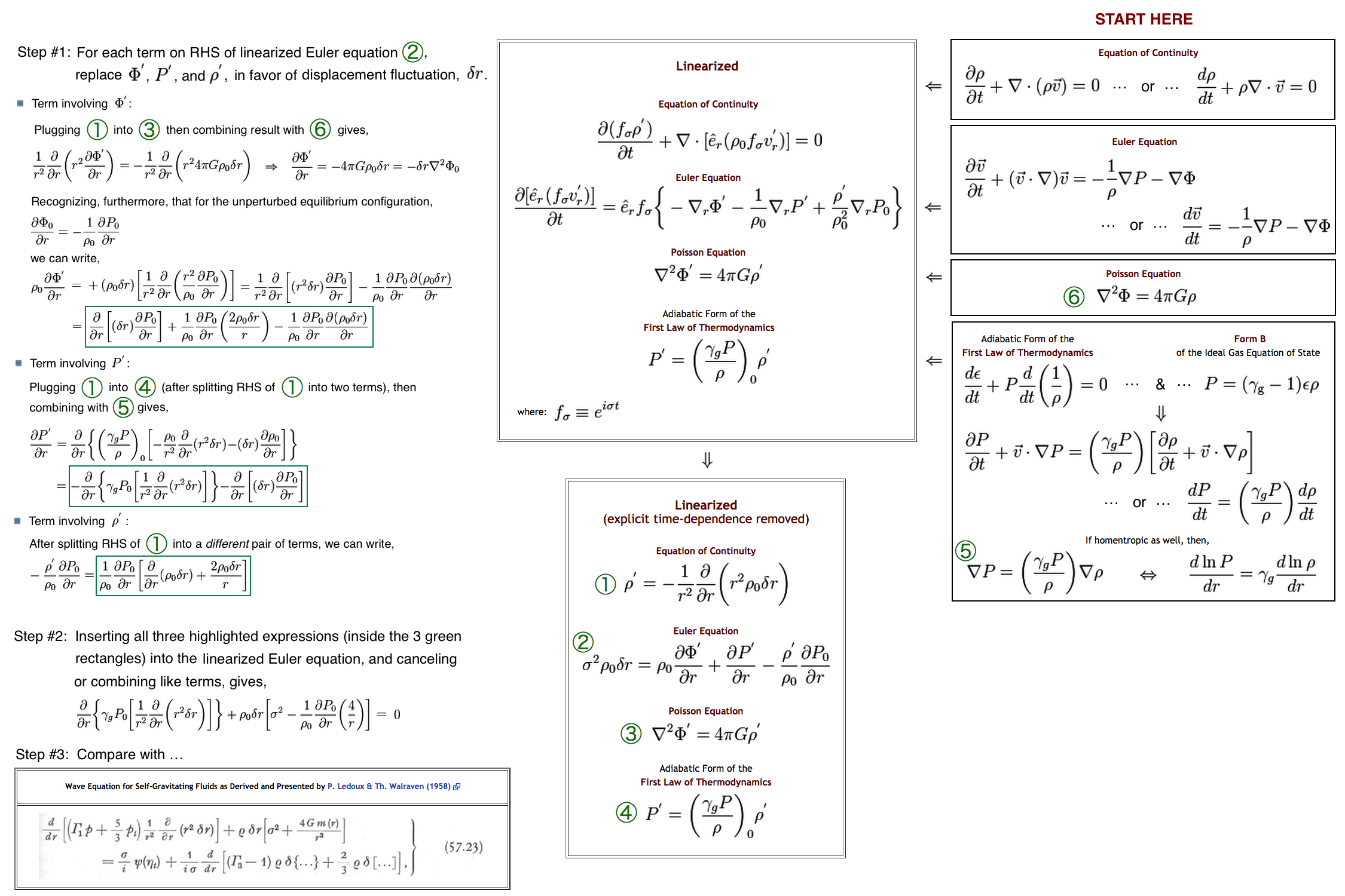
|
<math>~\frac{\delta\rho}{\rho_c} </math> |
<math>~=</math> |
<math>~- \frac{1}{r^2}\frac{d}{d r} \biggl[ r^3 \biggl(\frac{\rho}{\rho_c}\biggr) \frac{\delta r}{r_0} \biggr] </math> |
|
|
<math>~=</math> |
<math>~- \frac{1}{\xi^2}\frac{d}{d \xi} \biggl[ \xi^3 \biggl(\frac{\rho}{\rho_c}\biggr) x \biggr]\, .</math> |
Hence, we can write,
|
<math>~\frac{1}{\xi^2} \frac{dg}{d\xi}</math> |
<math>~=</math> |
<math>~- \frac{1}{\xi^2}\frac{d}{d \xi} \biggl[ \xi^3 \biggl(\frac{\rho}{\rho_c}\biggr) x \biggr] </math> |
|
<math>~\Rightarrow~~~ g</math> |
<math>~=</math> |
<math>~- \xi^3 \biggl(\frac{\rho}{\rho_c}\biggr) x </math> |
|
<math>~\Rightarrow~~~ x</math> |
<math>~=</math> |
<math>~- \frac{g}{\xi^3}~ e^{\psi} \, . </math> |
So, in terms of the radial displacement function, the eigenfunction for the marginally unstable configuration that has the Bonnor-Ebert limiting mass is,
|
<math>~x_Y</math> |
<math>~=</math> |
<math>~- \frac{g_Y}{\xi^3}~ e^{\psi} </math> |
|
|
<math>~=</math> |
<math>~- \biggl[\frac{1}{\xi} \frac{d\psi}{d\xi} - e^{-\psi}\biggr]e^{\psi} \, .</math> |
Verification of Analytic Solution
Yabushita (1975) states that the radial eigenfunction for the marginally unstable isothermal configuration is (see his equation 5.6),
|
<math>~x </math> |
<math>~=</math> |
<math>~\biggl[ \frac{\psi '}{\xi} - e^{-\psi}\biggr] e^{\psi} \, .</math> |
As we have just demonstrated, this expression for the displacement function is, indeed, equivalent to the expression that was derived by Yabushita (1974) for the perturbation function, <math>~g_Y</math>. (The overall sign has been reversed on the expression, but this leading factor of negative one is arbitrary.) In order to see if this, indeed, satisfies the
Isothermal LAWE with <math>~\sigma_c^2=0</math>
|
<math>~0</math> |
<math>~=</math> |
<math>~ \frac{d^2x}{d\xi^2} + \biggl[4 - \xi \psi ' \biggr] \frac{1}{\xi} \cdot \frac{dx}{d\xi} + \biggl[ \frac{\psi ' }{\xi} \biggr] x \, , </math> |
we need to evaluate the first and second derivatives of the eigenfunction. We also need to keep in mind that from the isothermal Lane-Emden equation, we know that,
|
<math>~\frac{1}{\xi^2} \frac{d}{d\xi}\biggr[ \xi^2 \psi ' \biggr]</math> |
<math>~=</math> |
<math>~e^{-\psi}</math> |
|
<math>~\Rightarrow ~~~ \psi </math> |
<math>~=</math> |
<math>~e^{-\psi} - \frac{2 \psi '}{\xi} \, .</math> |
So, the first derivative of the eigenfunction is,
|
<math>~\frac{dx}{d\xi}</math> |
<math>~=</math> |
<math>~\frac{d}{d\xi} \biggl\{ \biggl[ \frac{\psi '}{\xi} - e^{-\psi}\biggr] e^{\psi} \biggr\}</math> |
|
|
<math>~=</math> |
<math>~ \biggl[ \frac{\psi '}{\xi} - e^{-\psi}\biggr] \psi ' e^{\psi} + \biggl[ \frac{\psi }{\xi} - \frac{\psi '}{\xi^2} + \psi ' e^{-\psi}\biggr] e^{\psi} </math> |
|
|
<math>~=</math> |
<math>~\biggl\{ \biggl[ \frac{\psi '}{\xi} - e^{-\psi}\biggr] \psi ' + \biggl[ \frac{1}{\xi}\biggl( e^{-\psi} - \frac{2 \psi '}{\xi} \biggr) - \frac{\psi '}{\xi^2} + \psi ' e^{-\psi}\biggr] \biggr\} e^{\psi} </math> |
|
|
<math>~=</math> |
<math>~ \biggl[ \frac{(\psi ')^2}{\xi} - \frac{3\psi '}{\xi^2}\biggr]e^{\psi} + \frac{1}{\xi} \, . </math> |
And the second derivative is,
|
<math>\frac{d^2x}{d\xi^2}</math> |
<math>~=</math> |
<math>~ \frac{d}{d\xi}\biggl\{\biggl[\frac{(\psi ')^2}{\xi} - \frac{3\psi '}{\xi^2}\biggr]e^{\psi} + \frac{1}{\xi} \biggr\} </math> |
|
|
<math>~=</math> |
<math>~ \biggl[\frac{(\psi ')^2}{\xi} - \frac{3\psi '}{\xi^2}\biggr] \psi ' e^{\psi} +e^{\psi} \biggl\{\biggl[\frac{2\psi ' \psi }{\xi} - \frac{(\psi ')^2}{\xi^2} \biggr] -\biggl[ \frac{3\psi }{\xi^2} - \frac{6\psi '}{\xi^3}\biggr] \biggr\} - \frac{1}{\xi^2} </math> |
|
|
<math>~=</math> |
<math>~e^{\psi}\biggl\{ \frac{(\psi ')^3}{\xi} - \frac{4 (\psi ')^2}{\xi^2} + \frac{6\psi '}{\xi^3} + \biggl[ \frac{2\psi '}{\xi} - \frac{3}{\xi^2} \biggr]\psi \biggr\} - \frac{1}{\xi^2} </math> |
|
|
<math>~=</math> |
<math>~e^{\psi}\biggl\{ \frac{(\psi ')^3}{\xi} - \frac{4 (\psi ')^2}{\xi^2} + \frac{6\psi '}{\xi^3} - \biggl[ \frac{2\psi '}{\xi} - \frac{3}{\xi^2} \biggr] \frac{2 \psi '}{\xi} \biggr\} + \frac{2\psi '}{\xi} - \frac{4}{\xi^2} </math> |
|
|
<math>~=</math> |
<math>~ e^{\psi}\biggl\{ \frac{(\psi ')^3}{\xi} - \frac{8 (\psi ')^2}{\xi^2} + \frac{12\psi '}{\xi^3} \biggr\}+ \frac{2\psi '}{\xi} - \frac{4}{\xi^2} \, . </math> |
Plugging these expressions into the isothermal LAWE, we have,
|
<math>~ \frac{d^2x}{d\xi^2} + \biggl[4 - \xi \psi ' \biggr] \frac{1}{\xi} \cdot \frac{dx}{d\xi} + \biggl[\frac{\psi ' }{\xi} \biggr] x </math> |
<math>~=</math> |
<math>~ e^{\psi}\biggl\{ \frac{(\psi ')^3}{\xi} - \frac{8 (\psi ')^2}{\xi^2} + \frac{12\psi '}{\xi^3} \biggr\}+ \frac{2\psi '}{\xi} - \frac{4}{\xi^2} </math> |
|
|
|
<math>~ + \biggl[\frac{4}{\xi} - \psi ' \biggr] \biggl\{ \biggl[ \frac{(\psi ')^2}{\xi} - \frac{3\psi '}{\xi^2}\biggr]e^{\psi} + \frac{1}{\xi}\biggr\} + \frac{\psi ' }{\xi} \biggl\{ \biggl[ \frac{\psi '}{\xi} - e^{-\psi}\biggr] e^{\psi} \biggr\} </math> |
|
|
<math>~=</math> |
<math>~ e^{\psi}\biggl\{ \frac{(\psi ')^3}{\xi} - \frac{8 (\psi ')^2}{\xi^2} + \frac{12\psi '}{\xi^3} + \biggl(\frac{\psi '}{\xi} \biggr)^2 + \biggl[\frac{4}{\xi} - \psi ' \biggr] \cdot\biggl[ \frac{(\psi ')^2}{\xi} - \frac{3\psi '}{\xi^2}\biggr] \biggr\} </math> |
|
|
|
<math>~ + \frac{1}{\xi}\biggl[\frac{4}{\xi} - \psi ' \biggr] - \frac{\psi ' }{\xi} + \frac{2\psi '}{\xi} - \frac{4}{\xi^2} </math> |
|
|
<math>~=</math> |
<math>~ e^{\psi}\biggl\{ \frac{(\psi ')^3}{\xi} - \frac{8 (\psi ')^2}{\xi^2} + \frac{12\psi '}{\xi^3} + \biggl(\frac{\psi '}{\xi} \biggr)^2 + \frac{4(\psi ')^2}{\xi^2} - \frac{12\psi '}{\xi^3} - \frac{(\psi ')^3}{\xi} + \frac{3(\psi ')^2}{\xi^2} \biggr\} </math> |
|
|
<math>~=</math> |
<math>~ 0 \, . </math> |
Amazing!!
Actually, we should have started with the simpler version of the expression for the displacement function, namely,
|
<math>~x </math> |
<math>~=</math> |
<math>~1 - \frac{\psi ' e^\psi}{\xi} </math> |
|
<math>~\Rightarrow ~~~ \frac{dx}{d\xi} </math> |
<math>~=</math> |
<math>~- \biggl\{ \frac{\psi e^\psi}{\xi} + \frac{(\psi ')^2 e^\psi}{\xi} - \frac{\psi ' e^\psi}{\xi^2} \biggr\}</math> |
|
|
<math>~=</math> |
<math>~- \biggl\{ \frac{e^\psi}{\xi}\biggl[ e^{-\psi} - \frac{2 \psi '}{\xi} \biggr] + \frac{(\psi ')^2 e^\psi}{\xi} - \frac{\psi ' e^\psi}{\xi^2} \biggr\}</math> |
|
|
<math>~=</math> |
<math>~- \biggl\{ \frac{1}{\xi} + \frac{(\psi ')^2 e^\psi}{\xi} - \frac{3\psi ' e^\psi}{\xi^2} \biggr\}</math> |
|
<math>~\Rightarrow ~~~ - \frac{d\ln x}{d\ln\xi} </math> |
<math>~=</math> |
<math>~\frac{1}{x}\biggl\{ 1 + (\psi ')^2 e^\psi - \frac{3\psi ' e^\psi}{\xi} \biggr\}</math> |
|
|
<math>~=</math> |
<math>~\frac{1}{x}\biggl[ (\psi ')^2 e^\psi + 3x-2\biggr] \, .</math> |
Hence, if at the surface we impose a boundary condition, <math>~d\ln x/d\ln\xi = -3</math>, then this also means that, at the surface,
|
<math>~3x_\mathrm{surf}</math> |
<math>~=</math> |
<math>~\biggl[ (\psi ')^2 e^\psi + 3x-2\biggr]_\mathrm{surf} </math> |
|
<math>~\Rightarrow~~~ \biggl[ (\psi ')^2 e^\psi \biggr]_\mathrm{surf} </math> |
<math>~=</math> |
<math>~2 \, .</math> |
And this is precisely the condition that Bonnor recognized was associated with the critical turning point along the equilibrium sequence. Hence, we can now also precisely associate the marginally (dynamically) unstable configuration as being the configuration at the turning point.
For the record, it would also be good to know what the limiting value of the Yabushita displacement function is at the center of the isothermal configuration. Drawing on some of our already-developed power-series expressions, we have,
|
<math>~x </math> |
<math>~=</math> |
<math>~1 - \frac{\psi ' e^\psi}{\xi} </math> |
|
|
<math>~=</math> |
<math>~1 - \frac{1}{\xi} \biggl[1 + \psi + \frac{\psi^2}{2} \cdots \biggr] \frac{d}{d\xi}\biggl[ \psi \biggr] </math> |
|
|
<math>~\approx</math> |
<math>~1 - \frac{1}{\xi} \biggl[1 + \biggl(\frac{\xi^2}{6} - \frac{\xi^4}{120}\biggr) + \frac{1}{2} \biggl(\frac{\xi^2}{6} - \frac{\xi^4}{120}\biggr)^2 \biggr] \frac{d}{d\xi}\biggl[ \frac{\xi^2}{6} - \frac{\xi^4}{120} \biggr] </math> |
|
|
<math>~\approx</math> |
<math>~1 - \biggl[1 + \frac{\xi^2}{6} \biggr] \biggl[ \frac{1}{3} - \frac{\xi^2}{30} \biggr] </math> |
|
|
<math>~\approx</math> |
<math>~1 - \biggl[ \frac{1}{3} - \frac{\xi^2}{30} \biggr] +\frac{\xi^2}{18} </math> |
|
|
<math>~\approx</math> |
<math>~\frac{2}{3} + \frac{2^2\xi^2}{3^2 \cdot 5} \, . </math> |
Try to Generalize
Derivation of Polytropic Displacement Function
| iPhone snapshot of "whiteboard" Eureka! moment. |
 |
Now, let's turn our attention to the,
Polytropic LAWE
|
|
<math>~0 = \frac{d^2x}{d\xi^2} + \biggl[ 4 - (n+1) Q \biggr] \frac{1}{\xi} \cdot \frac{dx}{d\xi} + (n+1) \biggl[ \biggl( \frac{\sigma_c^2}{6\gamma_g } \biggr) \frac{\xi^2}{\theta} - \alpha Q\biggr] \frac{x}{\xi^2} </math> |
|
where: <math>~Q(\xi) \equiv - \frac{d\ln\theta}{d\ln\xi} \, ,</math> <math>~\sigma_c^2 \equiv \frac{3\omega^2}{2\pi G\rho_c} \, ,</math> and, <math>~\alpha \equiv \biggl(3 - \frac{4}{\gamma_\mathrm{g}}\biggr)</math> |
|
Based on the analytic expression that Yabushita (1975) derived for the isothermal case, plus some "white board" poking around, the following general polytropic displacement function looks promising:
|
<math>~x</math> |
<math>~=</math> |
<math>~1 + \biggl(\frac{n-3}{n-1}\biggr) \frac{\theta^' }{\xi \theta^{n}} \, .</math> |
Keeping in mind that, according to the polytropic Lane-Emden equation,
|
<math>~\theta^{}</math> |
<math>~=</math> |
<math>~- \theta^n - \frac{2\theta^'}{\xi} \, ,</math> |
the first derivative is,
|
<math>~\frac{dx}{d\xi}</math> |
<math>~=</math> |
<math>~\biggl(\frac{n-3}{n-1}\biggr) \biggl\{ \frac{\theta^{} }{\xi \theta^{n}} - \frac{n(\theta^')^2 }{\xi \theta^{n+1}} - \frac{\theta^' }{\xi^2 \theta^{n}} \biggr\} </math> |
|
|
<math>~=</math> |
<math>~\biggl(\frac{3-n}{n-1}\biggr) \biggl\{ \frac{1}{\xi \theta^{n}}\biggl[\theta^n + \frac{2\theta^'}{\xi} \biggr] + \frac{n(\theta^')^2 }{\xi \theta^{n+1}} + \frac{\theta^' }{\xi^2 \theta^{n}} \biggr\} </math> |
|
|
<math>~=</math> |
<math>~ \biggl(\frac{3-n}{n-1}\biggr) \biggl\{ \frac{1}{\xi} + \frac{n(\theta^')^2 }{\xi \theta^{n+1}} + \frac{3\theta^' }{\xi^2 \theta^{n}} \biggr\} \, ; </math> |
and the second derivative is,
|
<math>\frac{d^2 x}{d\xi^2}</math> |
<math>~=</math> |
<math>~\biggl(\frac{3-n}{n-1}\biggr) \biggl\{ -\frac{1}{\xi^2} + \frac{2n(\theta^')\theta^{} }{\xi \theta^{n+1}} - \frac{n(\theta^')^2 }{\xi^2 \theta^{n+1}} - (n+1) \frac{n(\theta^')^3 }{\xi \theta^{n+2}} + \frac{3\theta^{} }{\xi^2 \theta^{n}} - \frac{6\theta^' }{\xi^3 \theta^{n}} - \frac{3n (\theta^')^2 }{\xi^2 \theta^{n+1}} \biggr\} </math> |
|
|
<math>~=</math> |
<math>~\biggl(\frac{n-3}{n-1}\biggr) \biggl\{ \frac{1}{\xi^2} + \bigg[ \frac{2n(\theta^')}{\xi \theta^{n+1}} + \frac{3 }{\xi^2 \theta^{n}} \biggr] \biggl[ \theta^n + \frac{2\theta^'}{\xi} \biggr] + (n+1) \frac{n(\theta^')^3 }{\xi \theta^{n+2}} + \frac{6\theta^' }{\xi^3 \theta^{n}} + \frac{4n (\theta^')^2 }{\xi^2 \theta^{n+1}} \biggr\} </math> |
|
|
<math>~=</math> |
<math>~\biggl(\frac{n-3}{n-1}\biggr) \biggl\{ \frac{1}{\xi^2} + \frac{2n(\theta^')}{\xi \theta} + \frac{3 }{\xi^2 } + \frac{4n(\theta^')^2}{\xi^2 \theta^{n+1}} + \frac{6\theta^' }{\xi^3 \theta^{n}} + (n+1) \frac{n(\theta^')^3 }{\xi \theta^{n+2}} + \frac{6\theta^' }{\xi^3 \theta^{n}} + \frac{4n (\theta^')^2 }{\xi^2 \theta^{n+1}} \biggr\} </math> |
|
|
<math>~=</math> |
<math>~ \biggl(\frac{n-3}{n-1}\biggr) \biggl\{ \frac{4}{\xi^2} + \frac{2n(\theta^')}{\xi \theta} + \frac{12\theta^' }{\xi^3 \theta^{n}}+ \frac{8n(\theta^')^2}{\xi^2 \theta^{n+1}} + (n+1) \frac{n(\theta^')^3 }{\xi \theta^{n+2}} \biggr\} \, . </math> |
Hence, setting <math>~\sigma_c^2 = 0</math> in the polytropic LAWE gives,
|
LAWE |
<math>~=</math> |
<math>~ \frac{d^2x}{d\xi^2} + \biggl[ 4 + (n+1) \biggl(\frac{\xi \theta^'}{\theta} \biggr) \biggr] \frac{1}{\xi} \cdot \frac{dx}{d\xi} + \alpha (n+1) \biggl(\frac{\xi \theta^'}{\theta} \biggr) \frac{x}{\xi^2} </math> |
|
|
<math>~=</math> |
<math>~ \biggl(\frac{n-3}{n-1}\biggr) \biggl\{ \frac{4}{\xi^2} + \frac{2n(\theta^')}{\xi \theta} + \frac{12\theta^' }{\xi^3 \theta^{n}}+ \frac{8n(\theta^')^2}{\xi^2 \theta^{n+1}} + (n+1) \frac{n(\theta^')^3 }{\xi \theta^{n+2}} \biggr\} </math> |
|
|
|
<math>~ - \biggl(\frac{n-3}{n-1}\biggr) \biggl[ 4 + (n+1) \biggl(\frac{\xi \theta^'}{\theta} \biggr) \biggr] \biggl[ \frac{1}{\xi^2} + \frac{n(\theta^')^2 }{\xi^2 \theta^{n+1}} + \frac{3\theta^' }{\xi^3 \theta^{n}} \biggr] + \alpha (n+1) \biggl(\frac{\theta^'}{\xi \theta} \biggr) \biggl[ 1 + \biggl(\frac{n-3}{n-1}\biggr) \frac{\theta^' }{\xi \theta^{n}} \biggr] </math> |
|
|
<math>~=</math> |
<math>~\alpha (n+1) \biggl(\frac{\theta^'}{\xi \theta} \biggr) + \biggl(\frac{n-3}{n-1}\biggr) \biggl\{ \frac{4}{\xi^2} + \frac{2n(\theta^')}{\xi \theta} + \frac{12\theta^' }{\xi^3 \theta^{n}}+ \frac{8n(\theta^')^2}{\xi^2 \theta^{n+1}} + (n+1) \frac{n(\theta^')^3 }{\xi \theta^{n+2}} - \frac{4}{\xi^2} - \frac{4n(\theta^')^2 }{\xi^2 \theta^{n+1}} - \frac{12\theta^' }{\xi^3 \theta^{n}} </math> |
|
|
|
<math>~ - (n+1) \biggl(\frac{ \theta^'}{\xi\theta} \biggr) - (n+1) \biggl[ \frac{n(\theta^')^3 }{\xi \theta^{n+2}} \biggr] - (n+1) \biggl[ \frac{3 (\theta^')^2 }{\xi^2 \theta^{n+1}} \biggr] + \alpha (n+1) \biggl[ \frac{(\theta^')^2 }{\xi^2 \theta^{n+1}} \biggr] \biggr\} </math> |
|
|
<math>~=</math> |
<math>~\alpha (n+1) \biggl(\frac{\theta^'}{\xi \theta} \biggr) + \biggl(\frac{n-3}{n-1}\biggr) \biggl\{ (n-1) \biggl(\frac{ \theta^'}{\xi\theta} \biggr) + \frac{(\theta^')^2}{\xi^2 \theta^{n+1}} \biggl[4n - 3(n+1) + \alpha (n+1) \biggr]\biggr\} </math> |
|
|
<math>~=</math> |
<math>~[ \alpha (n+1) + (n-3) ] \biggl[ \biggl(\frac{ \theta^'}{\xi\theta} \biggr) + \biggl(\frac{n-3}{n-1}\biggr) \frac{(\theta^')^2}{\xi^2 \theta^{n+1}} \biggr] </math> |
|
|
<math>~=</math> |
<math>~[ \alpha (n+1) + (n-3) ] \biggl[ 1 + \biggl(\frac{n-3}{n-1}\biggr) \frac{\theta^'}{\xi \theta^{n}} \biggr] \biggl(\frac{ \theta^'}{\xi\theta} \biggr) </math> |
|
|
<math>~=</math> |
<math>~- [ \alpha (n+1) + (n-3) ] \biggl(\frac{x}{\xi^2} \biggr) Q \, . </math> |
Hence, if <math>~\gamma = (n+1)/n</math>, then, <math>~\alpha = (3-4/\gamma) = (3-n)/(n+1)</math>, and the polytropic LAWE is satisfied. HOOOORAAAAY! (18 March 2017)
Behavior of First Logarithmic Derivative
For the record, let's develop an expression for the logarithmic derivative of this displacement function.
|
<math>~\frac{d\ln x}{d\ln \xi} = \frac{\xi}{x} \cdot \frac{dx}{d\xi}</math> |
<math>~=</math> |
<math>~ \biggl(\frac{3-n}{n-1}\biggr) \biggl[ 1 + \frac{n(\theta^')^2 }{\theta^{n+1}} + \frac{3\theta^' }{\xi \theta^{n}} \biggr] \biggl[ 1 + \biggl(\frac{n-3}{n-1}\biggr) \frac{\theta^' }{\xi \theta^{n}} \biggr]^{-1} </math> |
|
|
<math>~=</math> |
<math>~ - (n-3) \biggl[ 1 + \frac{n(\theta^')^2 }{\theta^{n+1}} + \frac{3\theta^' }{\xi \theta^{n}} \biggr] \biggl[ (n-1) + (n-3) \frac{\theta^' }{\xi \theta^{n}} \biggr]^{-1} </math> |
|
<math>~\Rightarrow ~~~ \biggl[ (n-1) + (n-3) \frac{\theta^' }{\xi \theta^{n}} \biggr] \frac{d\ln x}{d\ln \xi} </math> |
<math>~=</math> |
<math>~ - (n-3) \biggl[ 1 + \frac{n(\theta^')^2 }{\theta^{n+1}} + \frac{3\theta^' }{\xi \theta^{n}} \biggr] </math> |
|
<math>~\Rightarrow ~~~ \biggl[ (n-1) \biggr] \frac{d\ln x}{d\ln \xi} </math> |
<math>~=</math> |
<math>~ - (n-3) \biggl\{ \biggl[ 1 + \frac{n(\theta^')^2 }{\theta^{n+1}} + \frac{3\theta^' }{\xi \theta^{n}} \biggr] + \biggl[ \frac{\theta^' }{\xi \theta^{n}} \biggr] \frac{d\ln x}{d\ln \xi} \biggr\} </math> |
|
|
<math>~=</math> |
<math>~ - (n-3) \biggl\{ \biggl[ 1 + \frac{n(\theta^')^2 }{\theta^{n+1}} \biggr] + \biggl[ \frac{\theta^' }{\xi \theta^{n}} \biggr] \biggl[3 + \frac{d\ln x}{d\ln \xi}\biggr] \biggr\} </math> |
Now, as we have discussed above, Yabushita (1992) has argued that for pressure-truncated configurations, the appropriate surface boundary condition should be,
<math>\frac{d\ln x}{d\ln\xi} = -3 \, .</math>
If we adopt this surface boundary condition, then this just-derived expression becomes,
|
<math>~3 (n-1) </math> |
<math>~=</math> |
<math>~ (n-3) \biggl[ 1 + \frac{n(\theta^')^2 }{\theta^{n+1}} \biggr] </math> |
|
<math>~\Rightarrow~~~ (n-3) \biggl[ \frac{n(\theta^')^2 }{\theta^{n+1}} \biggr] </math> |
<math>~=</math> |
<math>~ 2n </math> |
|
<math>~\Rightarrow~~~ \frac{(\theta^')^2 }{\theta^{n+1}} </math> |
<math>~=</math> |
<math>~ \frac{2 }{(n-3) } \, . </math> |
According to Horedt (1970), this is precisely the functional condition that pinpoints the <math>~P_e</math>-max turning point(s) along the equilibrium sequence in a <math>~P-V</math> diagram, for all pressure-truncated, polytropic spheres with <math>~n \ge 3</math>. And, according to Kimura (1981), this is precisely the functional condition that pinpoints the maximum mass turning point(s) along equlibrium sequences as displayed in a mass-radius diagram.
Behavior Approaching Center
It would also be good to know what the limiting value of this displacement function is at the center of the polytropic configuration. Drawing on some of our already-developed power-series expressions, we have,
|
<math>~x </math> |
<math>~=</math> |
<math>~1 + \biggl(\frac{n-3}{n-1}\biggr) \frac{\theta^' }{\xi \theta^{n}} \, .</math> |
|
|
<math>~=</math> |
<math>~1 + \biggl(\frac{n-3}{n-1}\biggr)\frac{1}{\xi} \biggl[1- \frac{\xi^2}{6} + \frac{n\xi^4}{120} + \cdots \biggr]^{-n} \frac{d}{d\xi}\biggl[1- \frac{\xi^2}{6} + \frac{n\xi^4}{120} + \cdots \biggr] </math> |
|
|
<math>~\approx</math> |
<math>~1 + \biggl(\frac{n-3}{n-1}\biggr) \biggl[1 + \frac{n\xi^2}{6} \biggr] \biggl[- \frac{1}{3} + \frac{n\xi^2}{30} \biggr] </math> |
|
|
<math>~\approx</math> |
<math>~1 - \frac{1}{3}\cdot \biggl(\frac{n-3}{n-1}\biggr) \biggl[1 + \frac{n\xi^2}{15} \biggr] </math> |
So, let's rescale the polytropic displacement function such that the central value is unity for all values of the polytropic index. We have,
|
<math>~x_P</math> |
<math>~\equiv</math> |
<math>~A_0 \biggl[ 1 + \biggl(\frac{n-3}{n-1}\biggr) \frac{\theta^' }{\xi \theta^{n}} \biggr] \, ,</math> |
where,
|
<math>~A_0</math> |
<math>~\equiv</math> |
<math>~\biggl[ 1 - \frac{1}{3}\cdot \biggl(\frac{n-3}{n-1}\biggr) \biggr]^{-1} </math> |
|
|
<math>~=</math> |
<math>~\biggl[ \frac{3(n-1)- (n-3)}{3(n-1)} \biggr]^{-1} </math> |
|
|
<math>~=</math> |
<math>~\frac{3(n-1)}{2n} \, . </math> |
Note that this even provides the correct normalization factor for the isothermal case <math>~(n=\infty)</math>.

Material that appears after this point in our presentation is under development and therefore
may contain incorrect mathematical equations and/or physical misinterpretations.
| Go Home |
What if Eigenfrequency not Zero
Here we should keep in mind that the conventional surface boundary condition is,
|
<math>~\frac{d\ln x}{d\ln\xi}</math> |
<math>~=</math> |
<math>~\frac{1}{\gamma_\mathrm{g}} \biggl( 4 - 3\gamma_\mathrm{g} + \frac{\omega^2 R^3}{GM_\mathrm{tot}} \biggr)</math> |
Recalling that the ratio of the mean to central density is given by the structural form factor,
|
<math>~\frac{\bar\rho}{\rho_c} = f_\mathrm{M}</math> |
<math>~=</math> |
<math>~\biggl( - \frac{3\theta^'}{\xi} \biggr) \, ,</math> |
we can write,
|
<math>~\frac{\omega^2 R^3}{GM_\mathrm{tot}}</math> |
<math>~=</math> |
<math>~ \frac{\omega^2 R^3}{G}\biggl(\frac{3}{4\pi \bar\rho R^3} \biggr) </math> |
|
|
<math>~=</math> |
<math>~ \frac{3\omega^2 }{4\pi G}\biggl[\rho_c\biggl( - \frac{3\theta^'}{\xi} \biggr) \biggr]^{-1} </math> |
|
|
<math>~=</math> |
<math>~ \sigma_c^2 \biggl( - \frac{\xi}{6\theta^'} \biggr) \, , </math> |
where,
<math>~\sigma_c^2 \equiv \frac{3\omega^2}{2\pi G\rho_c} \, .</math>
Hence, the conventional surface boundary can be written as,
|
<math>~-~\frac{d\ln x}{d\ln\xi}</math> |
<math>~=</math> |
<math>~\alpha + \frac{\sigma_c^2}{6 \gamma_\mathrm{g}} \biggl( \frac{\xi}{\theta^'} \biggr) </math> |
|
|
<math>~=</math> |
<math>~ \biggl[ \biggl( \frac{\sigma_c^2}{6 \gamma_\mathrm{g}}\biggr) \frac{\xi^2}{\theta} -\alpha Q \biggr] \frac{\theta}{\xi \theta^'} </math> |
|
|
<math>~0 = \frac{d^2x}{d\xi^2} + \biggl[ 4 - (n+1) Q \biggr] \frac{1}{\xi} \cdot \frac{dx}{d\xi} + (n+1) \biggl[ \biggl( \frac{\sigma_c^2}{6\gamma_g } \biggr) \frac{\xi^2}{\theta} - \alpha Q\biggr] \frac{x}{\xi^2} </math> |
|
where: <math>~Q(\xi) \equiv - \frac{d\ln\theta}{d\ln\xi} \, ,</math> <math>~\sigma_c^2 \equiv \frac{3\omega^2}{2\pi G\rho_c} \, ,</math> and, <math>~\alpha \equiv \biggl(3 - \frac{4}{\gamma_\mathrm{g}}\biggr)</math> |
|
Now, if we return to the above derivation but, this time, do not set <math>~\sigma_c^2 = 0</math>, the polytropic LAWE gives,
|
LAWE |
<math>~=</math> |
<math>~ \frac{d^2x}{d\xi^2} + \biggl[ 4 + (n+1) \biggl(\frac{\xi \theta^'}{\theta} \biggr) \biggr] \frac{1}{\xi} \cdot \frac{dx}{d\xi} + \alpha (n+1) \biggl(\frac{\xi \theta^'}{\theta} \biggr) \frac{x}{\xi^2} + \biggl( \frac{\sigma_c^2}{6}\biggr) \frac{n x}{\theta} </math> |
|
|
<math>~=</math> |
<math>~ \biggl(\frac{n-3}{n-1}\biggr) \biggl\{ \frac{4}{\xi^2} + \frac{2n(\theta^')}{\xi \theta} + \frac{12\theta^' }{\xi^3 \theta^{n}}+ \frac{8n(\theta^')^2}{\xi^2 \theta^{n+1}} + (n+1) \frac{n(\theta^')^3 }{\xi \theta^{n+2}} \biggr\} </math> |
|
|
|
<math>~ - \biggl(\frac{n-3}{n-1}\biggr) \biggl[ 4 + (n+1) \biggl(\frac{\xi \theta^'}{\theta} \biggr) \biggr] \biggl[ \frac{1}{\xi^2} + \frac{n(\theta^')^2 }{\xi^2 \theta^{n+1}} + \frac{3\theta^' }{\xi^3 \theta^{n}} \biggr] + \alpha (n+1) \biggl(\frac{\theta^'}{\xi \theta} \biggr) \biggl[ 1 + \biggl(\frac{n-3}{n-1}\biggr) \frac{\theta^' }{\xi \theta^{n}} \biggr] + \biggl( \frac{\sigma_c^2}{6}\biggr) \frac{n}{\theta}\biggl[ 1 + \biggl(\frac{n-3}{n-1}\biggr) \frac{\theta^' }{\xi \theta^{n}} \biggr] </math> |
|
|
<math>~=</math> |
<math>~\alpha (n+1) \biggl(\frac{\theta^'}{\xi \theta} \biggr) + \biggl(\frac{n-3}{n-1}\biggr) \biggl\{ \frac{4}{\xi^2} + \frac{2n(\theta^')}{\xi \theta} + \frac{12\theta^' }{\xi^3 \theta^{n}}+ \frac{8n(\theta^')^2}{\xi^2 \theta^{n+1}} + (n+1) \frac{n(\theta^')^3 }{\xi \theta^{n+2}} - \frac{4}{\xi^2} - \frac{4n(\theta^')^2 }{\xi^2 \theta^{n+1}} - \frac{12\theta^' }{\xi^3 \theta^{n}} </math> |
|
|
|
<math>~ - (n+1) \biggl(\frac{ \theta^'}{\xi\theta} \biggr) - (n+1) \biggl[ \frac{n(\theta^')^3 }{\xi \theta^{n+2}} \biggr] - (n+1) \biggl[ \frac{3 (\theta^')^2 }{\xi^2 \theta^{n+1}} \biggr] + \alpha (n+1) \biggl[ \frac{(\theta^')^2 }{\xi^2 \theta^{n+1}} \biggr] \biggr\} + \biggl( \frac{\sigma_c^2}{6}\biggr) \frac{n}{\theta}\biggl[ 1 + \biggl(\frac{n-3}{n-1}\biggr) \frac{\theta^' }{\xi \theta^{n}} \biggr] </math> |
|
|
<math>~=</math> |
<math>~\alpha (n+1) \biggl(\frac{\theta^'}{\xi \theta} \biggr) + \biggl(\frac{n-3}{n-1}\biggr) \biggl\{ (n-1) \biggl(\frac{ \theta^'}{\xi\theta} \biggr) + \frac{(\theta^')^2}{\xi^2 \theta^{n+1}} \biggl[4n - 3(n+1) + \alpha (n+1) \biggr]\biggr\} + \biggl( \frac{\sigma_c^2}{6}\biggr) \frac{n}{\theta}\biggl[ 1 + \biggl(\frac{n-3}{n-1}\biggr) \frac{\theta^' }{\xi \theta^{n}} \biggr] </math> |
|
|
<math>~=</math> |
<math>~\biggl[ \alpha (n+1) + (n-3) \biggr] \biggl[ \biggl(\frac{ \theta^'}{\xi\theta} \biggr) + \biggl( \frac{n-3}{n-1}\biggr) \frac{(\theta^')^2}{\xi^2 \theta^{n+1}} \biggr] + \biggl( \frac{\sigma_c^2}{6}\biggr) \frac{n}{\theta}\biggl[ 1 + \biggl(\frac{n-3}{n-1}\biggr) \frac{\theta^' }{\xi \theta^{n}} \biggr] </math> |
|
|
<math>~=</math> |
<math>~\biggl[ \alpha (n+1) + (n-3) \biggr] \biggl(\frac{ \theta^'}{\xi\theta} \biggr)\biggl[ 1 + \biggl( \frac{n-3}{n-1}\biggr) \frac{\theta^'}{\xi \theta^{n}} \biggr] + \biggl( \frac{\sigma_c^2}{6}\biggr) \frac{n}{\theta}\biggl[ 1 + \biggl(\frac{n-3}{n-1}\biggr) \frac{\theta^' }{\xi \theta^{n}} \biggr] </math> |
|
|
<math>~=</math> |
<math>~ \biggl[ 1 + \biggl( \frac{n-3}{n-1}\biggr) \frac{\theta^'}{\xi \theta^{n}} \biggr] \biggl\{[ \alpha (n+1) + (n-3) ] \biggl(\frac{ \theta^'}{\xi\theta} \biggr) + \biggl( \frac{\sigma_c^2}{6}\biggr) \frac{n}{\theta}\biggr\} </math> |
|
|
<math>~=</math> |
<math>~ \frac{x}{\xi^2} \biggl\{[ \alpha (n+1) + (n-3) ] \biggl(\frac{ \xi \theta^'}{\theta} \biggr) + \biggl( \frac{\sigma_c^2}{6}\biggr) \frac{n\xi^2 }{\theta}\biggr\} </math> |
|
|
<math>~=</math> |
<math>~ \frac{x}{\xi^2} \biggl\{ \biggl( \frac{\sigma_c^2}{6}\biggr) \frac{n\xi^2 }{\theta} - [ \alpha (n+1) + (n-3) ] Q \biggr\} </math> |
References
Here we have drawn primarily from the following three sources:
- §5.3.8 (p. 372) of Horedt's (2004) treatise on Polytropes: Applications in Astrophysics and Related Fields
- S. Yabushita (1968, MNRAS, 140, 109) — Jeans's Type Gravitational Instability of Finite Isothermal Gas Spheres
- L. G. Taff & H. M. Horn (1974, MNRAS, 168, 427-432) — Radial Pulsations of Finite Isothermal Gas Spheres
See also:
- S. Yabushita (1975, MNRAS, 171, 85) — Jeans's Type Gravitational Instability of Finite Isothermal Gas Spheres — II
- S. Yabushita (1992, Astrophys. & Space Sciences, 193, 173 - 183) — Similarity between the structure and stability of isothermal and polytropic gas spheres
- J. P. Chieze (1987, A&A, 171, 225 - 232) — The fragmentation of molecular clouds. I - The mass-radius-velocity dispersion relations
- Radial Oscillations of Polytropic Spheres
- M. Lombardi & G. Bertin (2001, AA, 375, 1091-1099), Boyle's law and gravitational instability
- R. B. Larson (2003, Reports on Progress in Physics, 66, 1651-1697), The physics of star formation
- From G. P. Horedt (2013, ApJ, 773,131): "At present it is not clear whether the gravitational instability triggering the contraction of pre stellar cores is due to Jeans or Bonnor-Ebert instability (Padoan & Nordlund 2004, 2011; Hennebelle & Chabrier 2009).
- P. Padoan & A. Nordlund (2011, ApJL, 741, L22), The Observable Prestellar Phase of the Initial Mass Function. In the introduction, they state: Once a core mass grows beyond its Bonnor-Ebert mass, the core rapidly collapses within about a free-fall time …
- "Elmegreen (1999), for example, has proposed that the minimum stellar mass is of the order of this Bonnor-Ebert mass."
- Discussion of Bonnor-Ebert configurations
- On the Stability of non-isothermal Bonnor-Ebert spheres
- Power-point presentation focused on Bonnor-Ebert spheres
- Another power-point presentation
- Good, complimentary wiki discussion of BE spheres; includes dynamical collapse simulation.
- P. N. Foster and R. A. Chevalier (1993, ApJ, 416, 303), Gravitational Collapse of an Isothermal Sphere
|
|
|---|
|
© 2014 - 2021 by Joel E. Tohline |