Difference between revisions of "User:Tohline/Appendix/Ramblings/To Hadley and Imamura"
(Begin new chapter "Summary for Hadley & Imamura") |
(→Summary for Hadley & Imamura: Provide summary for Hadley and Imamura) |
||
| Line 2: | Line 2: | ||
<!-- __NOTOC__ will force TOC off --> | <!-- __NOTOC__ will force TOC off --> | ||
=Summary for Hadley & Imamura= | =Summary for Hadley & Imamura= | ||
This MediaWiki-based document is especially provided for Jimmy Imamura and Kathryn Hadley and summarizes the contents of a much longer [[User:Tohline/Appendix/Ramblings/Azimuthal_Distortions#Analyzing_Azimuthal_Distortions|set of technical notes that discusses the analysis of nonaxisymmetric distortions in rotating, self-gravitating fluids]]. | |||
{{LSU_HBook_header}} | {{LSU_HBook_header}} | ||
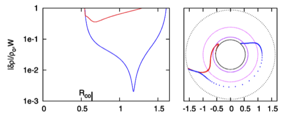
While studying the series of three papers that has recently been published by the [[#See_Also|Imamura & Hadley collaboration]], I was particularly drawn to the pair of plots presented in Figure 6 — and, again, in the top portion of Figure 13 and the top portion of Figure 16 — of [http://adsabs.harvard.edu/abs/2011Ap%26SS.334....1H HI11]. This pair of plots has been reprinted here, without modification, as our Figure 1. The curves delineated by the blue dots in this pair of [http://adsabs.harvard.edu/abs/2011Ap%26SS.334....1H HI11] plots display (on the left) the shape of the eigenfunction, <math>~f_1(\varpi)</math>, and (on the right) the "constant phase loci," <math>~\phi_1(\varpi)</math>, for an unstable, <math>~m=1</math> mode. In this case, the initial model for the depicted evolution is the equilibrium model from Table 2 of [http://adsabs.harvard.edu/abs/2011Ap%26SS.334....1H HI11] that has <math>~T/|W| = 0.253</math>; it is a fully self-gravitating torus with [[User:Tohline/SR#Barotropic_Structure|polytropic index]], <math>~n = 3/2</math>, and a rotation-law profile defined by a [[User:Tohline/AxisymmetricConfigurations/SolutionStrategies#Simple_Rotation_Profile_and_Centrifugal_Potential|"Keplerian" angular velocity profile]]. | |||
<div align="center"> | |||
<table border="1" cellpadding="3" align="center" width="75%"> | |||
<tr> | |||
<td align="center"> | |||
<b><font size="+1">Figure 1</font></b> | |||
</td> | |||
</tr> | |||
<tr><td align="center"> | |||
Panel pair extracted<sup>†</sup> without modification from the top-most segment of Figure 13, p. 18 of [http://adsabs.harvard.edu/abs/2011Ap%26SS.334....1H K. Hadley & J. N. Imamura (2011)]<p></p> | |||
"''Nonaxisymmetric Instabilities of Self-Gravitating Disks. ''I'' Toroids''"<p></p> | |||
''Astrophysics and Space Science'', 334, 1 - 26 © [http://www.springer.com/gp/about-springer/company-information/locations/springer-science-business-media-llc Springer Science+Business Media B.V.] | |||
</td></tr> | |||
<tr><td align="center"> | |||
[[File:ImamuraMontageTop.png|500px|Comparison with Hadley & Imamura (2011)]] | |||
</td></tr> | |||
<tr><td align="left"><sup>†</sup>This pair of plots also appears in the top portion of Figure 16 on p. 20 and, by itself, as Figure 6 on p. 12 of [http://adsabs.harvard.edu/abs/2011Ap%26SS.334....1H K. Hadley & J. N. Imamura (2011)].</td></tr> | |||
</table> | |||
</div> | |||
==Radial Eigenfunction== | |||
[[User:Tohline/Appendix/Ramblings/Azimuthal_Distortions#Radial_Eigenfunction|It occurred to me, first]], that the blue curve displayed in the left-hand panel of Figure 1 might be reasonably well approximated by piecing together a pair of arc-hyperbolic-tangent (ATANH) functions. In an effort to demonstrate this, I began by specifying a "midway" radial location, <math>~r_- < r_\mathrm{mid} < r_+ \, ,</math> at which the two ATANH functions meet and at which the density fluctuation is smallest. Then I defined a function of the form, | |||
<div align="center"> | |||
<table border="0" cellpadding="5" align="center"> | |||
<tr> | |||
<td align="center" bgcolor="blue"> </td> | |||
<td align="right"> | |||
<math>~f_\ln(\varpi)</math> | |||
</td> | |||
<td align="center"> | |||
<math>~=</math> | |||
</td> | |||
<td align="left"> | |||
<math>~\tanh^{-1}\biggl[1 - 2 \biggl( \frac{\varpi - r_-}{r_\mathrm{mid}-r_-} \biggr) \biggr]</math> | |||
</td> | |||
<td align="center"> | |||
for | |||
</td> | |||
<td align="left"> | |||
<math>r_- < \varpi < r_\mathrm{mid} \, ;</math> | |||
</td> | |||
</tr> | |||
<tr><td colspan="6" align="center">and</td></tr> | |||
<tr> | |||
<td align="center" bgcolor="green"> </td> | |||
<td align="right"> | |||
<math>~f_\ln(\varpi)</math> | |||
</td> | |||
<td align="center"> | |||
<math>~=</math> | |||
</td> | |||
<td align="left"> | |||
<math>~\tanh^{-1}\biggl[1 - 2 \biggl( \frac{\varpi - r_+}{r_\mathrm{mid}-r_+} \biggr) \biggr]</math> | |||
</td> | |||
<td align="center"> | |||
for | |||
</td> | |||
<td align="left"> | |||
<math>r_\mathrm{mid} < \varpi < r_+ \, .</math> | |||
</td> | |||
</tr> | |||
</table> | |||
</div> | |||
Recognizing that the figure depicting the [http://adsabs.harvard.edu/abs/2011Ap%26SS.334....1H HI11] eigenfunction is a semi-log plot, it seems clear that the relationship between our constructed function, <math>~f_\ln(\varpi)</math>, and the eigenfunction, <math>~f_1(\varpi)</math>, is, | |||
<div align="center"> | |||
<math>~f_1(\varpi) = e^{f_\ln(\varpi)} \, .</math> | |||
</div> | |||
[[User:Tohline/Appendix/Ramblings/Azimuthal_Distortions#SwitchToLog|Given that, in general, the following mathematical relation holds]], | |||
<div align="center"> | |||
<table border="0" cellpadding="5" align="center"> | |||
<tr> | |||
<td align="right"> | |||
<math>~\tanh^{-1}x</math> | |||
</td> | |||
<td align="center"> | |||
<math>~=</math> | |||
</td> | |||
<td align="left"> | |||
<math>~\ln\biggl( \frac{1+x}{1-x} \biggr)^{1/2} </math> | |||
</td> | |||
<td align="center"> | |||
for | |||
</td> | |||
<td align="left"> | |||
<math>x^2 < 1 \, .</math> | |||
</td> | |||
</tr> | |||
</table> | |||
</div> | |||
=== | for the innermost region of the toroidal configuration — that is, over the lower radial-coordinate range — <span id="SquareRoot">we can write,</span> | ||
<div align="center"> | |||
<table border="0" cellpadding="5" align="center"> | |||
<tr> | |||
<td align="center" bgcolor="blue"> </td> | |||
<td align="right"> | |||
<math>~f_1(\varpi) = e^{f_\ln(\varpi)}</math> | |||
</td> | |||
<td align="center"> | |||
<math>~=</math> | |||
</td> | |||
<td align="left"> | |||
<math>~\biggl( \frac{r_\mathrm{mid} - \varpi}{\varpi - r_-} \biggr)^{1/2} | |||
</math> | |||
</td> | |||
<td align="center"> | |||
for | |||
</td> | |||
<td align="left"> | |||
<math>r_- < \varpi < r_\mathrm{mid} \, .</math> | |||
</td> | |||
</tr> | |||
</table> | |||
</div> | |||
Similarly, we find that, over the upper radial-coordinate range, | |||
<div align="center"> | <div align="center"> | ||
<table border="0" cellpadding="5" align="center"> | <table border="0" cellpadding="5" align="center"> | ||
<tr> | <tr> | ||
<td align="center" bgcolor="green"> </td> | |||
<td align="right"> | <td align="right"> | ||
<math>~ | <math>~f_1(\varpi) = e^{f_\ln(\varpi)}</math> | ||
</td> | |||
<td align="center"> | |||
<math>~=</math> | |||
</td> | |||
<td align="left"> | |||
<math>~\biggl( \frac{r_\mathrm{mid} - \varpi}{\varpi - r_+} \biggr)^{1/2} | |||
</math> | |||
</td> | |||
<td align="center"> | |||
for | |||
</td> | |||
<td align="left"> | |||
<math>r_\mathrm{mid} < \varpi < r_+ \, .</math> | |||
</td> | |||
</tr> | |||
</table> | |||
</div> | |||
[[User:Tohline/Appendix/Ramblings/Azimuthal_Distortions#Playing_with_the_Radial_Eigenfunction|After a bit more experimentation]], we recognized that it is advantageous to replace the square root — that is, the exponent, ½ — with a variable exponent, <math>~p</math>, that can serve as an adjustable fitting parameter; and, in order to facilitate a degree of radial overlap between the two ATANH functions, we introduced different values of <math>~r_\mathrm{mid}</math> on the left and on the right. This led to a two-piece radial eigenfunction of the form, | |||
<div align="center"> | |||
<table border="0" cellpadding="5" align="center"> | |||
<tr> | |||
<td align="center" bgcolor="blue"> </td> | |||
<td align="right"> | |||
<math>~f_\mathrm{blue}(\varpi) </math> | |||
</td> | |||
<td align="center"> | |||
<math>~=</math> | |||
</td> | |||
<td align="left"> | |||
<math>~\biggl( \frac{r_\mathrm{blue} - \varpi}{\varpi - r_-} \biggr)^{p} | |||
</math> | |||
</td> | |||
<td align="center"> | |||
for | |||
</td> | |||
<td align="left"> | |||
<math>r_- < \varpi < r_\mathrm{blue} \, ,</math> | |||
</td> | |||
</tr> | |||
</table> | |||
</div> | |||
and, | |||
<div align="center"> | |||
<table border="0" cellpadding="5" align="center"> | |||
<tr> | |||
<td align="center" bgcolor="green"> </td> | |||
<td align="right"> | |||
<math>~f_\mathrm{green}(\varpi) </math> | |||
</td> | |||
<td align="center"> | |||
<math>~=</math> | |||
</td> | |||
<td align="left"> | |||
<math>~\biggl( \frac{r_\mathrm{green} - \varpi}{\varpi - r_+} \biggr)^{p} | |||
</math> | |||
</td> | |||
<td align="center"> | |||
for | |||
</td> | |||
<td align="left"> | |||
<math>r_\mathrm{green} < \varpi < r_+ \, ,</math> | |||
</td> | |||
</tr> | |||
</table> | |||
</div> | |||
where, <math>~r_\mathrm{mid}|_\mathrm{green} \le r_\mathrm{mid}|_\mathrm{blue}</math>. The expression that we are currently using for the radial eigenfunction is a sum of these two pieces, that is, | |||
<div align="center"> | |||
<table border="1" cellpadding="8" align="center"> | |||
<tr><td align="center"> | |||
<table border="0" cellpadding="5" align="center"> | |||
<tr> | |||
<td align="right"> | |||
<math>~f_1(\varpi)</math> | |||
</td> | |||
<td align="center"> | |||
<math>~=</math> | |||
</td> | |||
<td align="left"> | |||
<math>~f_\mathrm{green}(\varpi) + f_\mathrm{blue}(\varpi) \, . | |||
</math> | |||
</td> | |||
</tr> | |||
</table> | |||
</td></tr> | |||
</table> | |||
</div> | |||
For later use, we define from this function the minimum and maximum values, | |||
<div align="center"> | |||
<table border="0" cellpadding="5" align="center"> | |||
<tr> | |||
<td align="right"> | |||
<math>~[f_\ln]_\mathrm{min} \equiv \mathrm{min}[\ln(f_1)]</math> | |||
</td> | </td> | ||
<td align="center"> | <td align="center"> | ||
| |||
and | |||
| |||
</td> | </td> | ||
<td align="left"> | <td align="left"> | ||
<math>~ | <math>~[f_\ln]_\mathrm{max} \equiv \mathrm{max}[\ln(f_1)] \, .</math> | ||
</td> | </td> | ||
</tr> | </tr> | ||
</table> | </table> | ||
</div> | </div> | ||
==Constant Phase Loci== | |||
As is explained in [[User:Tohline/Appendix/Ramblings/Azimuthal_Distortions#Constant_Phase_Loci|our accompanying detailed technical notes]] — see, also [[User:Tohline/Appendix/Ramblings/Azimuthal_Distortions#Another_Improvement|another improvement]] — we have settled on the following prescription for the phase function, <math>~\phi_m(\varpi)</math>: | |||
<div align="center"> | <div align="center"> | ||
<table border="0" cellpadding="5" align="center"> | <table border="0" cellpadding="5" align="center"> | ||
| Line 44: | Line 270: | ||
</table> | </table> | ||
</div> | </div> | ||
where, <math>~\aleph</math> is a constant to be specified, | |||
<div align="center"> | |||
<table border="0" cellpadding="5" align="center"> | |||
<tr> | |||
<td align="right"> | |||
<math>~D_{1/2}(\varpi)</math> | |||
</td> | |||
<td align="center"> | |||
<math>~\equiv</math> | |||
</td> | |||
<td align="left"> | |||
<math>~\biggl[ \frac{f_\ln(\varpi) - [f_\ln]_\mathrm{min}}{[f_\ln]_\mathrm{max} - [f_\ln]_\mathrm{min}} \biggr]^{1/2} \, ,</math> | |||
</td> | |||
</tr> | |||
</table> | |||
</div> | |||
and, | |||
<div align="center"> | |||
<table border="0" cellpadding="5" align="center"> | |||
<tr> | |||
<td align="right"> | |||
<math>~f_\ln(\varpi)</math> | |||
</td> | |||
<td align="center"> | |||
<math>~\equiv</math> | |||
</td> | |||
<td align="left"> | |||
<math>~\ln[ f_1(\varpi)] \, .</math> | |||
</td> | |||
</tr> | |||
</table> | |||
</div> | |||
==Put It Together== | |||
<div align="center"> | <div align="center"> | ||
<table border="1"> | <table border="1"> | ||
<tr> | <tr> | ||
<td align="center" colspan="2"> | <td align="center" colspan="2"> | ||
<b><font size="+1">Figure | <b><font size="+1">Figure 2:</font></b> | ||
Radial and Azimuthal Eigenfunction Comparison | Radial and Azimuthal Eigenfunction Comparison | ||
</td> | </td> | ||
| Line 68: | Line 330: | ||
</table> | </table> | ||
</div> | </div> | ||
=See Also= | |||
* Imamura & Hadley collaboration: | |||
** [http://adsabs.harvard.edu/abs/2011Ap%26SS.334....1H K. Hadley & J. N. Imamura (2011, ''Astrophysics and Space Science'', 334, 1-26)], "Nonaxisymmetric instabilities in self-gravitating disks. I. Toroids" | |||
** [http://adsabs.harvard.edu/abs/2014Ap%26SS.353..191H K. Z. Hadley, P. Fernandez, J. N. Imamura, E. Keever, R. Tumblin, & W. Dumas (2014, ''Astrophysics and Space Science'', 353, 191-222)], "Nonaxisymmetric instabilities in self-gravitating disks. II. Linear and quasi-linear analyses" | |||
** [http://adsabs.harvard.edu/abs/2015Ap%26SS.359...10H K. Z. Hadley, W. Dumas, J. N. Imamura, E. Keever, & R. Tumblin (2015, ''Astrophysics and Space Science'', 359, article id. 10, 23 pp.)], "Nonaxisymmetric instabilities in self-gravitating disks. III. Angular momentum transport" | |||
{{LSU_HBook_footer}} | {{LSU_HBook_footer}} | ||
Revision as of 21:29, 2 February 2016
Summary for Hadley & Imamura
This MediaWiki-based document is especially provided for Jimmy Imamura and Kathryn Hadley and summarizes the contents of a much longer set of technical notes that discusses the analysis of nonaxisymmetric distortions in rotating, self-gravitating fluids.

|
|---|
| | Tiled Menu | Tables of Content | Banner Video | Tohline Home Page | |
While studying the series of three papers that has recently been published by the Imamura & Hadley collaboration, I was particularly drawn to the pair of plots presented in Figure 6 — and, again, in the top portion of Figure 13 and the top portion of Figure 16 — of HI11. This pair of plots has been reprinted here, without modification, as our Figure 1. The curves delineated by the blue dots in this pair of HI11 plots display (on the left) the shape of the eigenfunction, <math>~f_1(\varpi)</math>, and (on the right) the "constant phase loci," <math>~\phi_1(\varpi)</math>, for an unstable, <math>~m=1</math> mode. In this case, the initial model for the depicted evolution is the equilibrium model from Table 2 of HI11 that has <math>~T/|W| = 0.253</math>; it is a fully self-gravitating torus with polytropic index, <math>~n = 3/2</math>, and a rotation-law profile defined by a "Keplerian" angular velocity profile.
|
Figure 1 |
|
Panel pair extracted† without modification from the top-most segment of Figure 13, p. 18 of K. Hadley & J. N. Imamura (2011)
"Nonaxisymmetric Instabilities of Self-Gravitating Disks. I Toroids"
Astrophysics and Space Science, 334, 1 - 26 © Springer Science+Business Media B.V. |
| †This pair of plots also appears in the top portion of Figure 16 on p. 20 and, by itself, as Figure 6 on p. 12 of K. Hadley & J. N. Imamura (2011). |
Radial Eigenfunction
It occurred to me, first, that the blue curve displayed in the left-hand panel of Figure 1 might be reasonably well approximated by piecing together a pair of arc-hyperbolic-tangent (ATANH) functions. In an effort to demonstrate this, I began by specifying a "midway" radial location, <math>~r_- < r_\mathrm{mid} < r_+ \, ,</math> at which the two ATANH functions meet and at which the density fluctuation is smallest. Then I defined a function of the form,
|
<math>~f_\ln(\varpi)</math> |
<math>~=</math> |
<math>~\tanh^{-1}\biggl[1 - 2 \biggl( \frac{\varpi - r_-}{r_\mathrm{mid}-r_-} \biggr) \biggr]</math> |
for |
<math>r_- < \varpi < r_\mathrm{mid} \, ;</math> |
|
| and | |||||
|
<math>~f_\ln(\varpi)</math> |
<math>~=</math> |
<math>~\tanh^{-1}\biggl[1 - 2 \biggl( \frac{\varpi - r_+}{r_\mathrm{mid}-r_+} \biggr) \biggr]</math> |
for |
<math>r_\mathrm{mid} < \varpi < r_+ \, .</math> |
|
Recognizing that the figure depicting the HI11 eigenfunction is a semi-log plot, it seems clear that the relationship between our constructed function, <math>~f_\ln(\varpi)</math>, and the eigenfunction, <math>~f_1(\varpi)</math>, is,
<math>~f_1(\varpi) = e^{f_\ln(\varpi)} \, .</math>
Given that, in general, the following mathematical relation holds,
|
<math>~\tanh^{-1}x</math> |
<math>~=</math> |
<math>~\ln\biggl( \frac{1+x}{1-x} \biggr)^{1/2} </math> |
for |
<math>x^2 < 1 \, .</math> |
for the innermost region of the toroidal configuration — that is, over the lower radial-coordinate range — we can write,
|
<math>~f_1(\varpi) = e^{f_\ln(\varpi)}</math> |
<math>~=</math> |
<math>~\biggl( \frac{r_\mathrm{mid} - \varpi}{\varpi - r_-} \biggr)^{1/2} </math> |
for |
<math>r_- < \varpi < r_\mathrm{mid} \, .</math> |
Similarly, we find that, over the upper radial-coordinate range,
|
<math>~f_1(\varpi) = e^{f_\ln(\varpi)}</math> |
<math>~=</math> |
<math>~\biggl( \frac{r_\mathrm{mid} - \varpi}{\varpi - r_+} \biggr)^{1/2} </math> |
for |
<math>r_\mathrm{mid} < \varpi < r_+ \, .</math> |
After a bit more experimentation, we recognized that it is advantageous to replace the square root — that is, the exponent, ½ — with a variable exponent, <math>~p</math>, that can serve as an adjustable fitting parameter; and, in order to facilitate a degree of radial overlap between the two ATANH functions, we introduced different values of <math>~r_\mathrm{mid}</math> on the left and on the right. This led to a two-piece radial eigenfunction of the form,
|
<math>~f_\mathrm{blue}(\varpi) </math> |
<math>~=</math> |
<math>~\biggl( \frac{r_\mathrm{blue} - \varpi}{\varpi - r_-} \biggr)^{p} </math> |
for |
<math>r_- < \varpi < r_\mathrm{blue} \, ,</math> |
and,
|
<math>~f_\mathrm{green}(\varpi) </math> |
<math>~=</math> |
<math>~\biggl( \frac{r_\mathrm{green} - \varpi}{\varpi - r_+} \biggr)^{p} </math> |
for |
<math>r_\mathrm{green} < \varpi < r_+ \, ,</math> |
where, <math>~r_\mathrm{mid}|_\mathrm{green} \le r_\mathrm{mid}|_\mathrm{blue}</math>. The expression that we are currently using for the radial eigenfunction is a sum of these two pieces, that is,
|
For later use, we define from this function the minimum and maximum values,
|
<math>~[f_\ln]_\mathrm{min} \equiv \mathrm{min}[\ln(f_1)]</math> |
and |
<math>~[f_\ln]_\mathrm{max} \equiv \mathrm{max}[\ln(f_1)] \, .</math> |
Constant Phase Loci
As is explained in our accompanying detailed technical notes — see, also another improvement — we have settled on the following prescription for the phase function, <math>~\phi_m(\varpi)</math>:
|
<math>~m\phi_m</math> |
<math>~=</math> |
<math>~\tan^{-1}[\aleph \cdot D_{1/2}(\varpi)] \, .</math> |
where, <math>~\aleph</math> is a constant to be specified,
|
<math>~D_{1/2}(\varpi)</math> |
<math>~\equiv</math> |
<math>~\biggl[ \frac{f_\ln(\varpi) - [f_\ln]_\mathrm{min}}{[f_\ln]_\mathrm{max} - [f_\ln]_\mathrm{min}} \biggr]^{1/2} \, ,</math> |
and,
|
<math>~f_\ln(\varpi)</math> |
<math>~\equiv</math> |
<math>~\ln[ f_1(\varpi)] \, .</math> |
Put It Together
|
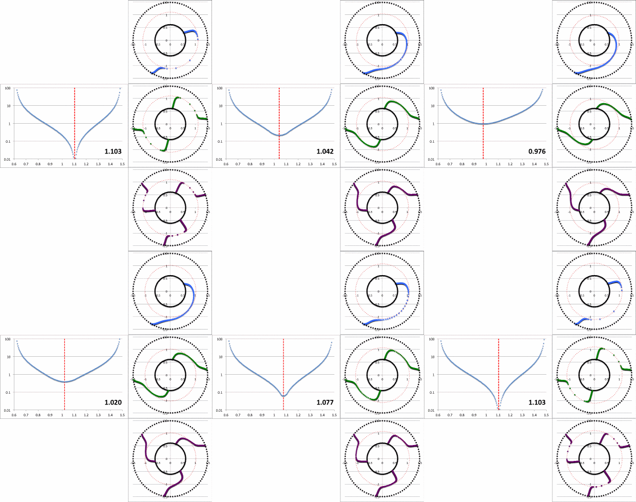
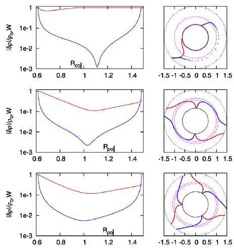
Figure 2: Radial and Azimuthal Eigenfunction Comparison |
|
| (a) Our Empirically Constructed Function | (b) Extracted from Figure 16 of HI11 |
See Also
- Imamura & Hadley collaboration:
- K. Hadley & J. N. Imamura (2011, Astrophysics and Space Science, 334, 1-26), "Nonaxisymmetric instabilities in self-gravitating disks. I. Toroids"
- K. Z. Hadley, P. Fernandez, J. N. Imamura, E. Keever, R. Tumblin, & W. Dumas (2014, Astrophysics and Space Science, 353, 191-222), "Nonaxisymmetric instabilities in self-gravitating disks. II. Linear and quasi-linear analyses"
- K. Z. Hadley, W. Dumas, J. N. Imamura, E. Keever, & R. Tumblin (2015, Astrophysics and Space Science, 359, article id. 10, 23 pp.), "Nonaxisymmetric instabilities in self-gravitating disks. III. Angular momentum transport"

|
|---|
|
© 2014 - 2021 by Joel E. Tohline |


