User:Tohline/Appendix/Ramblings/Nonlinar Oscillation

Radial Oscillations in Pressure-Truncated n = 5 Polytropes

[Comment by Joel Tohline on 24 August 2016]  Over the past few weeks, I have been putting together a powerpoint presentation that summarizes what I've learned, especially over the last several years, about turning points — and their relative positioning with respect to points of dynamical instability — along equilibrium sequences. One key finding, which is illustrated in Figure 3 of that discussion, is that the transition from stable to unstable systems along the n = 5 sequence occurs after, rather than at, the pressure maximum of the sequence. This means that, in the immediate vicinity of the pressure maximum, two stable equilibrium configurations exist with the same <math>~(K, M_\mathrm{tot}, P_e) </math> but different radii. Perhaps this means that, in the absence of dissipation, and without the need for a driving mechanism, a permanent oscillation between these two states can be activated.

Upon further thought, it occurred to me that a careful examination of the internal structure of both models — especially relative to one another — might reveal what the eigenvector of that (nonlinear) oscillation might be. In support of this idea, I point to the discussion of "Turning-Points and the Onset of Instability" found in §6.8 of [ST83] — specifically, on p. 149 in the paragraph that follows eq. (6.8.11) — where we find the following statement: "… the eigenfunction at a critical point is simply the Lagrangian displacement <math>~\xi</math> that carries an equilibrium configuration on the low-density side of the critical point into an equilibrium configuration on the high-density side."

See related arguments made by:

• Bisnovatyi-Kogan & Blinnikov (1974) — see especially their §6 — as we have briefly reviewed in an introductory paragraph
• Stahler (1983), as we have briefly reviewed in a separate chapter

Review of Internal Structure

Run of Mass

According to Chandrasekhar (Chapter IV, equation 67, p.97), the mass interior to <math>~\xi</math> is,

<math>~M(\xi)</math>

<math>~=</math>

<math>~4\pi a_n^3 \rho_c (-\xi^2 \theta^') \, .</math>

For a pressure-truncated polytrope, the total mass is,

<math>~M_\mathrm{tot}</math>

<math>~=</math>

<math>~4\pi a_n^3 \rho_c (-\tilde\xi^2 \tilde\theta^') \, ,</math>

which means that, as a function of <math>~\xi</math> in a pressure-truncated polytrope, the relative mass is,

<math>~m_\xi \equiv \frac{M(\xi)}{M_\mathrm{tot}}</math>	<math>~=</math>	<math>~\biggl[4\pi a_n^3 \rho_c (-\xi^2 \theta^') \biggr] \biggl[ 4\pi a_n^3 \rho_c (-\tilde\xi^2 \tilde\theta^') \biggr]^{-1}</math>
	<math>~=</math>	<math>~\frac{(-\xi^2 \theta^')}{(-\tilde\xi^2 \tilde\theta^')} \, .</math>

Thus, for an <math>~n = 5</math> system we have,

<math>~m_\xi</math>	<math>~=</math>	<math>~ \biggl(\frac{\xi}{\tilde\xi}\biggr)^2 \biggl[ \frac{\xi }{ 3}\biggl(1 + \frac{\xi^2}{3}\biggr)^{-3/2} \biggr] \biggl[ \frac{\tilde\xi }{ 3}\biggl(1 + \frac{\tilde\xi^2}{3}\biggr)^{-3/2} \biggr]^{-1}</math>
	<math>~=</math>	<math>~ \biggl(\frac{\xi}{\tilde\xi}\biggr)^3 \biggl(1 + \frac{\xi^2}{3}\biggr)^{-3/2} \biggl(1 + \frac{\tilde\xi^2}{3}\biggr)^{3/2} \, ;</math>

and, for the configuration at the pressure maximum <math>~(\tilde\xi = 3)</math>, in particular, we have,

<math>~m_0</math>

<math>~=</math>

<math>~\biggl(\frac{2\xi}{3}\biggr)^3 \biggl(1 + \frac{\xi^2}{3}\biggr)^{-3/2} \, .</math>

Corresponding Lagrangian Radial Coordinate

For any pressure-truncated polytrope, the fractional radial-coordinate running through the equilibrium configuration is,

<math>~\frac{r(\xi)}{R_\mathrm{eq}}</math>	<math>~=</math>	<math>~\frac{\xi}{\tilde\xi}</math>
<math>~\Rightarrow~~~ r(\xi)</math>	<math>~=</math>	<math>~\biggl(\frac{\xi}{\tilde\xi}\biggr) R_\mathrm{eq}</math>
<math>~\Rightarrow~~~r_\xi \equiv \frac{r(\xi)}{R_\mathrm{norm}}</math>	<math>~=</math>	<math>~\biggl(\frac{\xi}{\tilde\xi}\biggr) \biggl[ \frac{4\pi}{(n+1)^n}\biggr]^{1/(n-3)} \tilde\xi ( -\tilde\xi^2 \tilde\theta' )^{(1-n)/(n-3)} \, . </math>

For <math>~n=5</math> configurations, this means,

<math>~r_\xi</math>	<math>~=</math>	<math>~\biggl(\frac{\xi}{\tilde\xi}\biggr) \biggl[ \frac{4\pi}{2^5\cdot 3^5}\biggr]^{1/2} \tilde\xi ( -\tilde\xi^2 \tilde\theta' )^{-2} </math>
	<math>~=</math>	<math>~\xi \biggl\{ \biggl[ \frac{4\pi}{2^5\cdot 3^5}\biggr]^{1/2} \tilde\xi^{-4} \biggl[ \frac{\tilde\xi}{3} \biggl( 1+\frac{\tilde\xi^2}{3} \biggr)^{-3/2}\biggr]^{-2} \biggr\} </math>
	<math>~=</math>	<math>~\xi \biggl\{ \biggl[ \frac{4\pi}{2^5\cdot 3}\biggr]^{1/2} \tilde\xi^{-6} \biggl( 1+\frac{\tilde\xi^2}{3} \biggr)^{3}\biggr\} \, ; </math>

and, for the configuration at the pressure maximum <math>~(\tilde\xi = 3)</math>, in particular, this gives,

<math>~r_0</math>	<math>~=</math>	<math>~\xi \biggl\{ \biggl[ \frac{4\pi}{2^5\cdot 3}\biggr]^{1/2} \biggl(\frac{2}{3}\biggr)^6\biggr\} </math>
	<math>~=</math>	<math>~\xi \biggl[ \frac{2^9 \pi}{3^{13}}\biggr]^{1/2} </math>

Exploration

n = 5 Mass-Radius Relation

So, for any <math>~\tilde\xi</math> configuration, the parametric relationship between <math>~m_\xi</math> and <math>~r_\xi</math> in pressure-truncated, <math>~n=5</math> polytropes is,

<math>~m_\xi</math>	<math>~=</math>	<math>~ \biggl(\frac{\xi}{\tilde\xi}\biggr)^3 \biggl(1 + \frac{\xi^2}{3}\biggr)^{-3/2} \biggl(1 + \frac{\tilde\xi^2}{3}\biggr)^{3/2} \, ,</math>
<math>~r_\xi</math>	<math>~=</math>	<math>~\xi \biggl\{ \biggl[ \frac{4\pi}{2^5\cdot 3}\biggr]^{1/2} \tilde\xi^{-6} \biggl( 1+\frac{\tilde\xi^2}{3} \biggr)^{3}\biggr\} \, . </math>

And this can be inverted analytically in the case of <math>~\tilde\xi = 3</math>. Specifically,

<math>~m_0</math>	<math>~=</math>	<math>~\biggl(\frac{2\xi}{3}\biggr)^3 \biggl(1 + \frac{\xi^2}{3}\biggr)^{-3/2} </math>
<math>~\Rightarrow~~~ m_0^{2/3}</math>	<math>~=</math>	<math>~\biggl(\frac{2^2\xi^2}{3^2}\biggr) \biggl(1 + \frac{\xi^2}{3}\biggr)^{-1} </math>
<math>~\Rightarrow~~~ 2^2\xi^2 </math>	<math>~=</math>	<math>~ 3^2\biggl(1 + \frac{\xi^2}{3}\biggr) m_0^{2/3} </math>
<math>~\Rightarrow~~~ \xi^2 (2^2 - 3 m_0^{2/3}) </math>	<math>~=</math>	<math>~ 3^2m_0^{2/3} </math>
<math>~\Rightarrow~~~ \xi^2 </math>	<math>~=</math>	<math>~ \frac{3^2m_0^{2/3}}{(2^2 - 3 m_0^{2/3})} \, . </math>

Hence, the radius-mass relationship in the configuration at the <math>~P_\mathrm{max}</math> turning point is,

<math>~ r_0 (m_0) </math>

<math>~=</math>

<math>~\biggl[ \frac{2^9 \pi}{3^{13}}\biggr]^{1/2} \biggl[\frac{3^2m_0^{2/3}}{2^2 - 3 m_0^{2/3}}\biggr]^{1/2} \, . </math>

Actually, the inversion can be performed analytically for any choice of <math>~\tilde\xi</math> to obtain,

<math>~ r_\xi (m_\xi) </math>

<math>~=</math>

<math>~\tilde{r}_\mathrm{edge} \biggl[\frac{3^2m_\xi^{2/3}}{\tilde{C} - 3 m_\xi^{2/3}}\biggr]^{1/2} \, , </math>

where,

<math>~\tilde{C}</math>	<math>~\equiv</math>	<math>~ \frac{3^2}{\tilde\xi^2}\biggl( 1 + \frac{\tilde\xi^2}{3} \biggr) \, . </math>
<math>~\tilde{r}_\mathrm{edge}</math>	<math>~\equiv</math>	<math>~\biggl[ \frac{\pi}{2^3\cdot 3}\biggr]^{1/2} {\tilde\xi}^{-6} \biggl(1+\frac{\tilde\xi^2}{3}\biggr)^3 \, . </math>

Finite Difference Representation of Radial Eigenfunction

Preamble

<math>~\tilde{C}</math>	<math>~\equiv</math>	<math>~ \frac{3^2}{\tilde\xi^2}\biggl( 1 + \frac{\tilde\xi^2}{3} \biggr) \, , </math>
<math>~\tilde{r}_\mathrm{edge}</math>	<math>~\equiv</math>	<math>~ \biggl[ \frac{\pi}{2^3\cdot 3}\biggr]^{1/2} \biggl[ \frac{1}{ {\tilde\xi}^{2} }\biggl(1+\frac{\tilde\xi^2}{3}\biggr) \biggr] ^3 </math>
	<math>~=</math>	<math>~ \biggl[ \frac{\pi}{2^3\cdot 3}\biggr]^{1/2} \biggl[ \frac{\tilde{C} }{ 3^2 }\biggr] ^3 </math>
	<math>~=</math>	<math>~ \biggl[ \frac{\pi}{2^3\cdot 3^{13}}\biggr]^{1/2} {\tilde{C}}^3 \, . </math>

Note that when <math>~\tilde\xi = 3</math>,

<math>~\tilde{C}_3</math>	<math>~=</math>	<math>~ 4 \, , </math>
<math>~\tilde{r}_{e3}</math>	<math>~=</math>	<math>~ \biggl[ \frac{2^9\pi }{3^{13} } \biggr]^{1 / 2} \, . </math>

Conjectures

A first-cut examination of the structure of the radial eigenfunction associated with the <math>~P_\mathrm{max}</math> turning point is given by simply subtracting one <math>~r_\xi(m_\xi)</math> profile from another at the same applied external pressure. (The specific choices of the two appropriate values of <math>~\tilde\xi</math> are discussed in the subsection titled, "Configuration Pairing", which follows.) The answer appears to be,

<math>~[ \Delta r_\xi ]_{21} = [r_\xi (m_\xi)]_2 - [r_\xi (m_\xi)]_1 </math>	<math>~=</math>	<math>~ [\tilde{r}_\mathrm{edge}]_2 \biggl[\frac{3^2m_\xi^{2/3}}{\tilde{C}_2 - 3 m_\xi^{2/3}}\biggr]^{1/2} - [\tilde{r}_\mathrm{edge}]_1 \biggl[\frac{3^2m_\xi^{2/3}}{\tilde{C}_1 - 3 m_\xi^{2/3}}\biggr]^{1/2} </math>
	<math>~=</math>	<math>~ \biggl[ \frac{\pi}{2^3\cdot 3^{13}}\biggr]^{½} \biggl\{ {\tilde{C}_2}^3 \biggl[\frac{3^2m_\xi^{2/3}}{\tilde{C}_2 - 3 m_\xi^{2/3}}\biggr]^{1/2} - {\tilde{C}_1}^3 \biggl[\frac{3^2m_\xi^{2/3}}{\tilde{C}_1 - 3 m_\xi^{2/3}}\biggr]^{1 / 2} \biggr\} </math>
	<math>~=</math>	<math>~ \biggl[ \frac{\pi}{2^3\cdot 3^{13}}\biggr]^{1 / 2} \biggl\{ {\tilde{C}_2}^3 \biggl[\frac{3^2m_\xi^{2/3}/\tilde{C}_1 }{\tilde{C}_2/\tilde{C}_1 - 3 m_\xi^{2/3}/\tilde{C}_1 }\biggr]^{1 / 2} - {\tilde{C}_1}^3 \biggl[\frac{3^2m_\xi^{2/3}/\tilde{C}_1 }{1 - 3 m_\xi^{2/3}/\tilde{C}_1 }\biggr]^{1 / 2} \biggr\} </math>
	<math>~=</math>	<math>~ \biggl[ \frac{\pi}{2^3\cdot 3^{13}}\biggr]^{1 / 2} \biggl\{ {\tilde{C}_2}^3 \biggl[\frac{3/u }{\tilde{C}_2/\tilde{C}_1 - 1/u }\biggr]^{1 / 2} - {\tilde{C}_1}^3 \biggl[\frac{3/u }{1 - 1/u }\biggr]^{1 / 2} \biggr\} </math>
	<math>~=</math>	<math>~ {\tilde{C}_1}^3 \biggl[ \frac{\pi}{2^3\cdot 3^{12}}\biggr]^{1 / 2} \biggl\{ k_{21}^3 \biggl[\frac{1 }{k_{21} u - 1 }\biggr]^{1 / 2} - \biggl[\frac{1 }{u - 1 }\biggr]^{1 / 2} \biggr\} \, , </math>

where,

<math>~u \equiv \tilde{C}_1/(3 m_\xi^{2/3}) \, ,</math>

<math>~k_{21} \equiv \frac{ \tilde{C}_2 }{ \tilde{C}_1 } \, .</math>

After examining the form of this last expression, it is clear that we can also write,

<math>~[r_\xi (m_\xi)]_1</math>

<math>~=</math>

<math>~ {\tilde{C}_1}^3 \biggl[ \frac{\pi}{2^3\cdot 3^{12}}\biggr]^{1 / 2} \biggl[\frac{1 }{u - 1 }\biggr]^{1 / 2} \, , </math>

in which case, the lopsided fractional eigenfunction takes the form,

<math>~\frac{[ \Delta r_\xi ]_{21} }{[r_\xi (m_\xi)]_1} </math>

<math>~=</math>

<math>~ k_{21}^3 \biggl[\frac{u - 1 }{k_{21} u - 1 }\biggr]^{1 / 2} - 1 \, . </math>

And the centered fractional eigenfunction is,

<math>~\frac{[ \Delta r_\xi ]_{32} }{[r_\xi (m_\xi)]_1} </math>	<math>~=</math>	<math>~ \biggl\{ k_{31}^3 \biggl[\frac{u - 1 }{k_{31} u - 1 }\biggr]^{1 / 2} - 1 \biggr\} - \biggl\{ k_{21}^3 \biggl[\frac{u - 1 }{k_{21} u - 1 }\biggr]^{1 / 2} - 1 \biggr\} </math>
	<math>~=</math>	<math>~ k_{31}^3 \biggl[\frac{u - 1 }{k_{31} u - 1 }\biggr]^{1 / 2} - k_{21}^3 \biggl[\frac{u - 1 }{k_{21} u - 1 }\biggr]^{1 / 2} \, . </math>

Configuration Pairing

Setup

Now, let's identify two <math>~n=5</math> equilibrium states that sit very near the <math>~P_\mathrm{max}</math> turning point on the two separate branches of the equilibrium sequence and that have identical external pressures. We know from separate discussions that, in both cases,

<math> ~\frac{P_\mathrm{e}}{P_\mathrm{norm}} </math>	<math>~=~</math>	<math>~\biggl[ \frac{(n+1)^3}{4\pi}\biggr]^{(n+1)/(n-3)} \tilde\theta_n^{n+1}( -\tilde\xi^2 \tilde\theta' )^{2(n+1)/(n-3)} </math>
	<math>~=~</math>	<math>~\biggl[ \frac{2\cdot 3^3}{\pi}\biggr]^{3} \tilde\xi^{12} \tilde\theta_n^{6}( - \tilde\theta' )^{6} </math>
<math>~\Rightarrow~~~ \biggl[ \frac{\pi}{2\cdot 3^3}\biggr]^{1/2}\biggl[\frac{P_\mathrm{e}}{P_\mathrm{norm}}\biggr]^{1/6}</math>	<math>~=~</math>	<math>~ \tilde\xi^{2} \tilde\theta_n( - \tilde\theta' ) </math>
	<math>~=~</math>	<math>~ 3\ell^2 (1+\ell^2)^{-1/2} \frac{\ell}{\sqrt{3}} (1+\ell^2)^{-3/2} </math>
	<math>~=~</math>	<math>~ \sqrt{3}\ell^3 (1+\ell^2)^{-2} </math>

We can therefore write,

<math>~(1+\ell^2)^{2}</math>	<math>~=~</math>	<math>~ p_0\ell^3 </math>
<math>~\Rightarrow~~~\ell^4 - p_0\ell^3 + 2\ell^2 + 1</math>	<math>~=~</math>	<math>~ 0 \, , </math>

where,

<math>p_0 \equiv \biggl[ \frac{2\cdot 3^4}{\pi}\biggr]^{1/2}\biggl[\frac{P_\mathrm{e}}{P_\mathrm{norm}}\biggr]^{-1/6}</math>

So, in essence, we seek two real roots of this quartic equation that are near <math>~P_\mathrm{max}</math>, that is, that are near <math>~\ell = \sqrt{3}</math> — where <math>~p_0 = (2^8/3^3)^{1/2}</math>.

Because we are hunting for equilibrium configurations near <math>~P_\mathrm{max}</math>, it makes sense to make the variable substitution,

<math>~\ell</math>

<math>~\rightarrow</math>

<math>~\sqrt{3}(1+\epsilon) \, ,</math>

and look for pairs of values, <math>~\epsilon_\pm</math> (both real, but one positive and the other negative).

<math>~0</math>	<math>~=~</math>	<math>~3^2(1+\epsilon)^4 - 3^{3/2}p_0(1+\epsilon)^3 + 6(1+\epsilon)^2 + 1</math>
	<math>~=~</math>	<math>~ 3^2\biggl[1 + 4\epsilon + 6\epsilon^2 + 4\epsilon^3 + \epsilon^4\biggr] - 3^{3/2}p_0\biggl[ 1+ 3\epsilon + 3\epsilon^2 + \epsilon^3 )\biggr] + 6\biggl[1 + 2\epsilon + \epsilon^2\biggr] + 1 </math>
	<math>~=~</math>	<math>~ \epsilon^4 \biggl[ 9 \biggr] +\epsilon^3 \biggl[ 36 - 3^{3/2}p_0 \biggr] +\epsilon^2 \biggl[ 54 - 3^{5/2}p_0 + 6 \biggr] +\epsilon \biggl[36 - 3^{5/2}p_0 + 12 \biggr] +(16- 3^{3/2}p_0)\, . </math>

And, because we will only be examining values of the external pressure that are less than <math>~P_\mathrm{max}</math>, and we know that at the point of maximum pressure, <math>~3^{3/2}p_0 = 16</math>, it makes sense to make the substitution,

<math>~3^{3/2}p_0 ~~~\rightarrow ~~~ (16+\delta) \, .</math>

Hence, for a fixed choice of <math>~\delta </math> (reasonably small, and positive), we seek two real roots (one positive and the other negative) of the quartic relation,

<math>~0</math>	<math>~=~</math>	<math>~ 9\epsilon^4 +\epsilon^3 \biggl[ 36 - (16+\delta ) \biggr] +\epsilon^2 \biggl[ 60 - 3(16+\delta ) \biggr] +\epsilon \biggl[48 - 3(16+\delta ) \biggr] -\delta </math>
	<math>~=~</math>	<math>~ 9\epsilon^4 +\epsilon^3 (20-\delta ) +\epsilon^2 ( 12 - 3\delta ) -\epsilon (3\delta ) -\delta \, . </math>

What are the reasonable limits on <math>~\delta</math>? Well, first note that,

<math>~p_0</math>	<math>~=</math>	<math>~\frac{(1+\ell^2)^2}{\ell^3}</math>
<math>~\Rightarrow ~~~ 16+\delta </math>	<math>~=</math>	<math>~3^{3/2}\biggl[\frac{(1+\ell^2)^2}{\ell^3}\biggr]</math>
<math>~\Rightarrow ~~~ \delta </math>	<math>~=</math>	<math>~3^{3/2}\biggl[\frac{(1+\ell^2)^2}{\ell^3}\biggr] - 2^4 \, .</math>

Now, according to our accompanying discussion, the relevant limits on <math>~\ell</math> are <math>~\sqrt{3}</math> (set by the maximum pressure turning point) and 2.223175 (set by the transition to dynamical instability). The corresponding values of <math>~\delta </math> are:   0 (by design) and 0.69938.

Quartic Solution

Here, we will draw from the Wikipedia discussion of the quartic function. The generic form is,

<math>~0</math>

<math>~=</math>

<math>~ax^4 + bx^3 + cx^2 + dx + e \,.</math>

Relating this to our specific quartic function, we should ultimately make the following assignments:

<math>~a</math>	<math>~=</math>	<math>~9</math>
<math>~b</math>	<math>~=</math>	<math>~20 - \delta</math>
<math>~c</math>	<math>~=</math>	<math>~12 - 3\delta = 3(4-\delta )</math>
<math>~d</math>	<math>~=</math>	<math>~-3 \delta</math>
<math>~e</math>	<math>~=</math>	<math>~-\delta</math>

We need to evaluate the following expressions:

<math>~p</math>	<math>~\equiv</math>	<math>~\frac{8ac-3b^2}{8a^2}</math>
	<math>~=</math>	<math>~\frac{2^3 \cdot 3^3(4-\delta )-3(20-\delta )^2}{2^3\cdot 3^4}</math>
<math>~q</math>	<math>~\equiv</math>	<math>~\frac{b^3 - 4abc + 8a^2d}{8a^3}</math>
	<math>~=</math>	<math>~\frac{(20 - \delta )^3 - 2^2\cdot 3^3(4-\delta ) (20 - \delta ) - 2^3\cdot 3^5\delta }{2^3 \cdot 3^6}</math>
<math>~\Delta_0</math>	<math>~\equiv</math>	<math>~c^2 - 3bd + 12ae</math>
	<math>~=</math>	<math>~3^2(4-\delta )^2 + 3^2\delta (20 - \delta ) - 2^2\cdot 3^3\delta</math>
	<math>~=</math>	<math>~144</math>
<math>~\Delta_1</math>	<math>~\equiv</math>	<math>~2c^3 - 9bcd + 27b^2e+27ad^2 - 72ace</math>
	<math>~=</math>	<math>~2\cdot 3^3(4-\delta)^3 + 3^4(20-\delta)(4-\delta)\delta - 3^3(20-\delta)^2 \delta+3^7\delta^2 + 2^3\cdot 3^5(4-\delta)\delta</math>
	<math>~=</math>	<math>~3^3(128 + 32\delta + \delta^2) \, .</math>
Note:   <math>~\Delta_1^2 - 4\Delta_0^3</math>	<math>~=</math>	<math>~3^6(2^{13}\delta + 2^8\cdot 5 \delta^2 + 2^6\delta^3 + \delta^4) \, .</math>

For a given value of <math>~\delta</math>, then, the pair of real roots is:

<math>~\epsilon_\pm</math>

<math>~=</math>

<math>~ -\frac{b}{4a} + S \pm \frac{1}{2}\biggl[ -4S^2 - 2p - \frac{q}{S} \biggr]^{1/2} \, , </math>

where,

<math>~S</math>	<math>~\equiv</math>	<math>~ \frac{1}{2}\biggl[- \frac{2p}{3} + \frac{1}{3a}\biggl(Q + \frac{\Delta_0}{Q}\biggr) \biggr]^{1/2} \, , </math>
<math>~Q</math>	<math>~\equiv</math>	<math>~ \biggl[ \frac{\Delta_1 + \sqrt{\Delta_1^2 - 4\Delta_0^3}}{2} \biggr]^{1/3} \, . </math>

We have used an Excel spreadsheet to evaluate these expressions. The following table identifies <math>~\epsilon_\pm</math> pairs (the middle two columns of numbers) for twenty different values of the external pressure; more specifically, for twenty values of <math>~0 \le \delta \le 0.69938</math>, equally spaced between the two limits. The corresponding pairs of <math>~\tilde\xi_\pm</math> are also listed (rightmost pair of columns).

Table 1

Sets of Paired Models from Quartic Solution P_e/P_norm delta eps_+ eps_- xi_+ xi_- 160.867 0.00000 0.00000 0.00000 3.00000 3.00000 158.664 0.03681 0.05747 -0.05338 3.17241 2.83986 156.497 0.07362 0.08253 -0.07435 3.24759 2.77695 154.363 0.11043 0.10227 -0.09000 3.30681 2.72999 152.264 0.14724 0.11927 -0.10291 3.35781 2.69127 150.198 0.18405 0.13452 -0.11407 3.40355 2.65780 148.164 0.22086 0.14852 -0.12398 3.44556 2.62805 146.163 0.25767 0.16159 -0.13296 3.48476 2.60111 144.193 0.29448 0.17391 -0.14120 3.52174 2.57640 142.254 0.33129 0.18563 -0.14883 3.55690 2.55351 140.345 0.36809 0.19685 -0.15596 3.59055 2.53212 138.466 0.40490 0.20764 -0.16266 3.62291 2.51203 136.617 0.44171 0.21805 -0.16898 3.65415 2.49305 134.796 0.47852 0.22814 -0.17498 3.68442 2.47505 133.003 0.51533 0.23794 -0.18070 3.71382 2.45791 131.239 0.55214 0.24748 -0.18615 3.74245 2.44154 129.501 0.58895 0.25680 -0.19138 3.77039 2.42586 127.790 0.62576 0.26590 -0.19640 3.79770 2.41081 126.106 0.66257 0.27481 -0.20122 3.82444 2.39634 124.447 0.69938 0.28355 -0.20587 3.85065 2.38238

Two Example Eigenfunctions

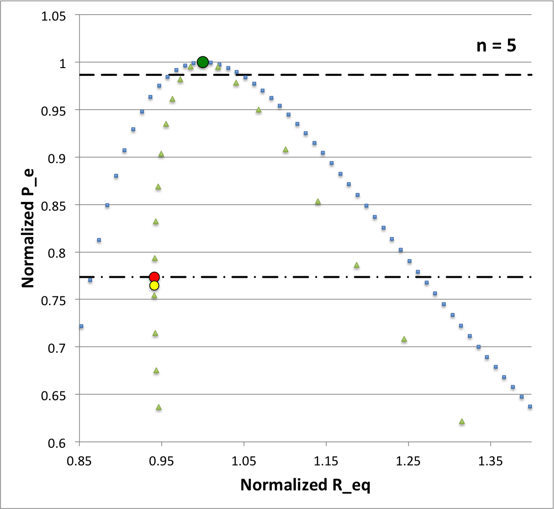
The following figure is fundamentally a reproduction of Figure 3 from an accompanying discussion. It presents the "Case M" equilibrium sequence from both an order-of-magnitude analysis (marked by light-blue squares) and a detailed force-balance analysis (light-green triangles). The dark green circular dot identifies the configuration at the pressure maximum of the sequence — <math>~P_\mathrm{max}/P_\mathrm{norm} = 160.867</math> — and the red circular dot identifies the location along the sequence where the transition from stable to dynamically unstable configurations occurs — <math>~P_e/P_\mathrm{norm} = 124.447</math>. (All pressures have been normalized to <math>~P_\mathrm{max}</math> in the figure.)

Figure 1

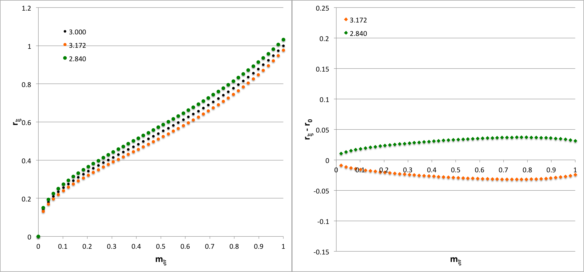
At any <math>~P_e</math> between these two limiting values, a pair of stable equilibrium configurations exist; approximately twenty example pairings are listed in Table 1. The horizontal, black dashed line in the figure has been drawn at <math>~P_e/P_\mathrm{norm} = 158.664</math>. The pair of equilibrium configurations associated with this pressure is identified graphically by the two points at which this dashed line intersects the detailed force-balance equilibrium sequence; as is detailed in the second row of Table 1, the configurations correspond to models having <math>~\tilde\xi = 2.83986</math> (right intersection) and <math>~\tilde\xi = 3.17241</math> (left intersection). The left-hand panel of Figure 2 shows how the Lagrangian radial coordinate varies with mass, <math>~r_\xi(m_\xi)</math>, throughout the interior of these two equilibrium configurations (the locus of green and orange dots, respectively); for reference, the profile of the configuration at <math>~P_\mathrm{max}</math> is presented as well (locus of black dots). The right-hand panel of Figure 2 shows the same paired configuration profiles, but relative to the profile of the configuration at <math>~P_\mathrm{max}</math>.

Figure 2

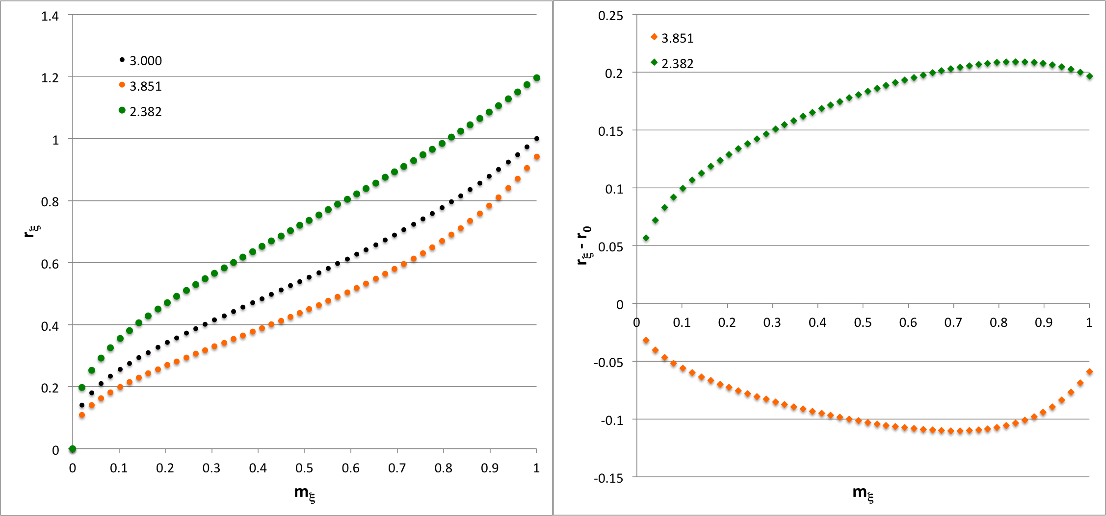
The horizontal, black dot-dash line in Figure 1 has been drawn at <math>~P_e/P_\mathrm{norm} = 124.447</math>. The pair of equilibrium configurations associated with this pressure is identified graphically by the two points at which this dot-dash line intersects the detailed force-balance equilibrium sequence; as is detailed in the last row of Table 1, the configurations correspond to models having <math>~\tilde\xi = 2.83986</math> (right intersection) and <math>~\tilde\xi = 3.17241</math> (left intersection), which is the configuration that marks the onset of a dynamical instability. The left-hand panel of Figure 3 shows how the Lagrangian radial coordinate varies with mass, <math>~r_\xi(m_\xi)</math>, throughout the interior of these two paired equilibrium configurations (the locus of green and orange dots, respectively); again, for reference, the profile of the configuration at <math>~P_\mathrm{max}</math> is presented as well (locus of black dots). The right-hand panel of Figure 3 shows the same paired configuration profiles, but relative to the profile of the configuration at <math>~P_\mathrm{max}</math>.

Figure 3

© 2014 - 2021 by Joel E. Tohline |   H_Book Home   |   YouTube   | Appendices: | Equations | Variables | References | Ramblings | Images | myphys.lsu | ADS | Recommended citation:   Tohline, Joel E. (2021), The Structure, Stability, & Dynamics of Self-Gravitating Fluids, a (MediaWiki-based) Vistrails.org publication, https://www.vistrails.org/index.php/User:Tohline/citation